Recursion and dynamic programming
This chapter covers
- Recognizing a problem that can be built from answers to smaller versions of itself
- Filling a table of answers from the smallest case upward
- Listing every subset of a set by exploring a tree of choices
- The longest increasing run hidden inside a list, in O(n log n)
- Choosing jobs that do not overlap, to earn the most
In chapter 1 you computed Fibonacci numbers three ways. The recursive version repeated work. The memoized version saved each answer in a table, and the loop version kept only the answers it still needed. That small example contains the whole idea of this chapter.
Dynamic programming is a way to solve a problem by answering smaller versions of the same problem first, saving those answers, and combining them. It applies when two things are true:
- The answer for a large input can be built from the answers for smaller inputs.
- The same smaller inputs come up again and again, so saving their answers avoids repeated work.
This chapter works through four problems. The first, making change with coins, is dynamic programming in its plainest form. The second, listing subsets, uses recursion without any saved answers. The last two combine dynamic programming with the sorting and searching you learned in chapter 3.
For each problem I first say, in one sentence, what one entry of the table means. That sentence is called the subproblem. Once it is written down, the code follows from it.
6.1 Making change with the fewest coins
The problem. You have coins of some values, as many of each as you like. What is the fewest number of coins that add up to a given amount? With coins 1, 2, and 5, the amount 11 needs three coins: 5 + 5 + 1. Some amounts cannot be made at all. With only a 2 coin, the amount 3 is impossible.
6.1.1 Why the obvious approach fails
A natural first try is to take the largest coin that fits, again and again. This is called a greedy approach. It works for 1, 2, and 5. It does not work for every set of coins (figure 6.1).
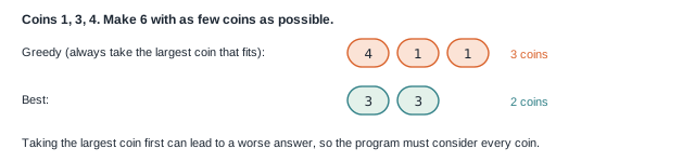
So the program has to consider every coin at every step. Trying every combination directly takes exponential time. Dynamic programming makes it fast.
6.1.2 The subproblem
Write down what one entry of the table means:
dp[t]is the fewest coins that add up to exactlyt.
Now think about the last coin used to make t. If that coin is c, the coins before it add up to t - c,
and the fewest coins for that is dp[t - c]. So using coin c last costs dp[t - c] + 1 coins. You do not
know which coin is last in the best answer, so try every coin and keep the smallest:
dp[t]= the smallest ofdp[t - c] + 1, over every coincthat is not larger thant.
The starting point is dp[0] = 0: zero coins make zero.
Fill the table by hand for the coins in figure 6.1, which are 1, 3, and 4, and the amount 6. Each row tries every coin that fits, and keeps the smallest count:
t | coins that fit | options from each coin | dp[t] |
|---|---|---|---|
| 1 | 1 | dp[0] + 1 = 1 | 1 |
| 2 | 1 | dp[1] + 1 = 2 | 2 |
| 3 | 1, 3 | dp[2] + 1 = 3, dp[0] + 1 = 1 | 1 |
| 4 | 1, 3, 4 | dp[3] + 1 = 2, dp[1] + 1 = 2, dp[0] + 1 = 1 | 1 |
| 5 | 1, 3, 4 | dp[4] + 1 = 2, dp[2] + 1 = 3, dp[1] + 1 = 2 | 2 |
| 6 | 1, 3, 4 | dp[5] + 1 = 3, dp[3] + 1 = 2, dp[2] + 1 = 3 | 2 |
dp[6] is 2, from 3 + 3. Greedy needed three coins for the same amount, because it took the 4 first and
never went back. The table records the best count for every smaller amount. Each new amount is then one
lookup plus one.
Two properties must hold for that to work. The answers must overlap, so that saving them avoids work.
dp[6] and dp[5] both read dp[1], and a longer table reads each entry many times. The best answer must
also be built from best answers to smaller amounts. Taking the smallest of dp[t - c] + 1 relies on that.
If some way of making t - c used fewer coins, dp[t - c] would hold that smaller number. When either
property fails, the table gives a wrong answer.
Because dp[t] only uses entries for smaller amounts, you can fill the table from left to right. Figure 6.2
shows the table for coins 1, 2, and 5, and how dp[11] is computed.
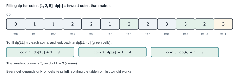
dp[11], the three coins lead back to dp[10], dp[9], and dp[6].dp[t] reads. The last part shows greedy choosing three coins where two are enough.6.1.3 The code
Listing 6.1 Coin change (lines 6 to 29). src/problems/dp.rs
pub fn coin_change(coins: &[i32], amount: i32) -> Option<i32> {
    if amount < 0 {
        return None;
    }

    let amount = amount as usize;
    let mut dp = vec![usize::MAX; amount + 1];
    dp[0] = 0;

    for total in 1..=amount {
        for &coin in coins {
            let coin = coin as usize;
            if coin > total || dp[total - coin] == usize::MAX {
                continue;
            }
            dp[total] = dp[total].min(dp[total - coin] + 1);
        }
    }

    match dp[amount] {
        usize::MAX => None,
        count => Some(count as i32),
    }
}
Read it against the recurrence:
- A negative amount is rejected first. After that check,
amount as usizecannot produce a strange value. vec![usize::MAX; amount + 1]creates the table, one entry per amount from 0 toamount.usize::MAX, the largestusize, stands for “cannot be made yet”.dp[0] = 0is the starting point.- The outer loop fills amounts from 1 upward. The inner loop tries every coin.
- The
continueskips a coin that is larger than the amount, or whose remainder cannot be made. The second check also preventsusize::MAX + 1, which would overflow. dp[total].min(dp[total - coin] + 1)keeps the smaller of the current best and the new option.
WARNING The second half of that continue is not an optimisation. Remove it and the function breaks.
If dp[total - coin] holds the sentinel, then dp[total - coin] + 1 adds one to the largest usize. A
debug build panics with “attempt to add with overflow”. A release build wraps around to 0, and the final
match reads 0 as a real count of zero coins. The table then reports fewer coins than exist. Add the
sentinel check before adding, or usize::MAX cannot stand for “impossible”.
At the end, a match turns the table entry into the result. The pattern usize::MAX matches that exact
value, meaning impossible, and returns None. Any other value is a count. So the function returns
Option<i32>, and the caller cannot mistake “impossible” for a number of coins.
The table has amount + 1 entries and each one tries every coin. The cost is O(amount × coins) time and
O(amount) memory.
Listing 6.2 The complete file. src/problems/dp.rs
//! Coin Change: minimum number of coins to make an amount.
//!
//! Classic dynamic programming. `Option<i32>` expresses "impossible" instead of
//! a magic `-1`.

pub fn coin_change(coins: &[i32], amount: i32) -> Option<i32> {
    if amount < 0 {
        return None;
    }

    let amount = amount as usize;
    let mut dp = vec![usize::MAX; amount + 1];
    dp[0] = 0;

    for total in 1..=amount {
        for &coin in coins {
            let coin = coin as usize;
            if coin > total || dp[total - coin] == usize::MAX {
                continue;
            }
            dp[total] = dp[total].min(dp[total - coin] + 1);
        }
    }

    match dp[amount] {
        usize::MAX => None,
        count => Some(count as i32),
    }
}

#[cfg(test)]
mod tests {
    use super::*;

    #[test]
    fn computes_minimum_coins() {
        assert_eq!(coin_change(&[1, 2, 5], 11), Some(3)); // 5 + 5 + 1
        assert_eq!(coin_change(&[2], 3), None);
        assert_eq!(coin_change(&[1], 0), Some(0));
    }
}
Run the tests with cargo test --lib coin_change. The tests check the example from section 6.1, an
impossible amount, and the amount 0.
6.2 Listing every subset
Not every recursive problem needs a table. Sometimes you need every possible answer, not the best one. Then recursion explores all the choices, and there is nothing to save.
The problem. List every subset of a set of distinct numbers. A subset is any selection of the
elements, including none of them and all of them. [1, 2, 3] has eight subsets: [], [1], [2], [3],
[1, 2], [1, 3], [2, 3], and [1, 2, 3].
The idea. Build subsets one element at a time. Start with the empty subset. From any subset, you can add
one more element, as long as it comes later in the input than the elements already chosen. That rule is what
stops [2, 1] from appearing as a copy of [1, 2]. Figure 6.3 draws the choices as a tree. Every node in
the tree is one subset.
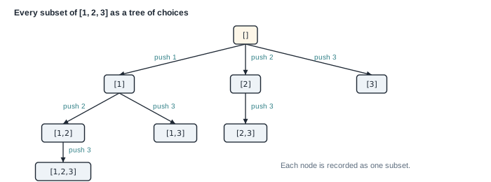
[1, 2, 3]. Each edge adds an element that comes after the last one chosen.To visit the whole tree, the program walks it depth first, going down one branch as far as it can before trying the next. Going down means adding an element; coming back up means removing it. This way of exploring choices is called backtracking.
start keeps [2, 1] out of the result.Listing 6.3 Subsets by backtracking. src/problems/backtracking.rs
//! Subsets: enumerate every subset of a set of distinct integers.
//!
//! Backtracking with clean `path.push(...)` + recursive exploration + `pop`.
//! `Vec<Vec<i32>>` is sorted in the tests to avoid order-dependent assertions.

pub fn subsets(nums: Vec<i32>) -> Vec<Vec<i32>> {
    let mut result = Vec::with_capacity(1 << nums.len());
    let mut path = Vec::new();

    fn backtrack(nums: &[i32], start: usize, path: &mut Vec<i32>, result: &mut Vec<Vec<i32>>) {
        result.push(path.clone());
        for idx in start..nums.len() {
            path.push(nums[idx]);
            backtrack(nums, idx + 1, path, result);
            path.pop();
        }
    }

    backtrack(&nums, 0, &mut path, &mut result);
    result
}

#[cfg(test)]
mod tests {
    use super::*;

    #[test]
    fn generates_all_subsets() {
        let mut subsets = subsets(vec![1, 2, 3]);
        subsets.sort_unstable();
        assert_eq!(subsets.len(), 8);
        assert!(subsets.contains(&vec![]));
        assert!(subsets.contains(&vec![1, 2, 3]));
    }

    #[test]
    fn empty_input_has_one_subset() {
        assert_eq!(subsets(vec![]), vec![vec![]]);
    }
}
backtrack is a function defined inside subsets, as go was in chapter 1. It takes four things:
nums, the input, borrowed.start, the first position it may choose from.path, the subset being built. Only onepathvector exists for the whole search, passed as&mut.result, the list of finished subsets, also passed as&mut.
On entry, backtrack records path.clone() in the result. The current path is one subset, the node of
the tree it has reached. Then, for each later position, it pushes that element, recurses to explore the
subtree below, and pops the element. After the pop, path is exactly as it was before the push, ready for
the next choice.
Trace the start of subsets(vec![1, 2, 3]):
| Call | path on entry | Records | Then pushes |
|---|---|---|---|
backtrack(start 0) | [] | [] | 1 |
backtrack(start 1) | [1] | [1] | 2 |
backtrack(start 2) | [1, 2] | [1, 2] | 3 |
backtrack(start 3) | [1, 2, 3] | [1, 2, 3] | nothing: the loop is empty |
back in start 2 | [1, 2] after pop | no more positions | |
back in start 1 | [1] after pop | 3 |
Vec::with_capacity(1 << nums.len()) reserves exactly enough room. 1 << n means 2 to the power n, because
shifting 1 left by n bits doubles it n times. A set of n elements has 2ⁿ subsets.
The work is O(n · 2ⁿ): there are 2ⁿ subsets and each clone copies up to n numbers. No algorithm can do better, because the output itself has that size.
6.3 The longest increasing run inside a list
The problem. In a list of numbers, pick some of them and keep their order. Each picked number must be
larger than the one before. What is the most you can pick? The picked numbers are called an increasing
subsequence. In [10, 9, 2, 5, 3, 7, 101, 18], you can pick 2, 3, 7, 18, so the answer is 4.
A subsequence may skip numbers. That is the difference from the substrings of chapter 3, which were contiguous.
The direct dynamic program. Let dp[i] be the length of the longest increasing subsequence that ends at
position i. For each i, look at every earlier j with a smaller number, and take the best dp[j] + 1. That is
O(n²), because each position looks at every earlier one.
A faster idea. Keep a different table, called tails. Its entries have this meaning:
The k-th smallest entry of
tailsis the smallest number that can end an increasing subsequence of length k.
Keeping the smallest possible ending number is useful because a smaller ending leaves more room for later numbers to extend it. When a new number arrives:
- If it is larger than every entry, it extends the longest subsequence found so far. Add it.
- Otherwise, find the smallest entry that is at least as large as it, and replace that entry with it. Some subsequence of that length can now end with a smaller number.
At the end, the number of entries is the answer. Figure 6.4 follows the example.
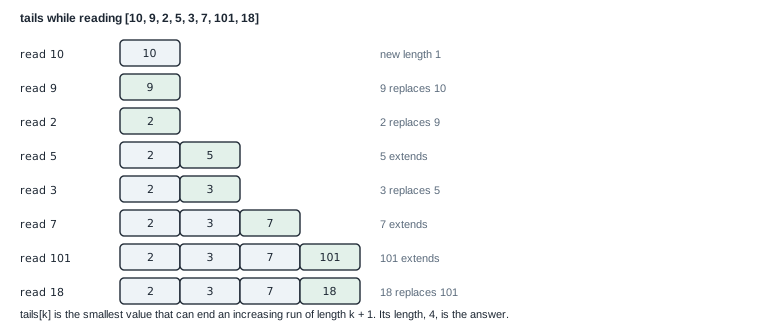
tails after each number. The green cell is the one that changed.Look at the last row. tails is 2, 3, 7, 18, which happens to be a real increasing subsequence here. That
is not true in general. tails can mix numbers from different subsequences. Only its length is meaningful.
The entries of tails are always in increasing order, so finding “the smallest entry at least as large” can
use a sorted structure. The program uses a BTreeSet, a set that keeps its elements sorted.
Listing 6.4 The complete program. src/bin/longest_increasing_subsequence.rs
use std::collections::BTreeSet;

fn lis_len(nums: &[i32]) -> usize {
    let mut tails = BTreeSet::new();

    for &num in nums {
        if let Some(&ceiling) = tails.range(num..).next() {
            tails.remove(&ceiling);
        }
        tails.insert(num);
    }

    tails.len()
}

fn main() {
    println!("{}", lis_len(&[10, 9, 2, 5, 3, 7, 101, 18])); // 4
    println!("{}", lis_len(&[0, 1, 0, 3, 2, 3])); // 4
    println!("{}", lis_len(&[7, 7, 7, 7])); // 1
    println!("{}", lis_len(&[5, 4, 3, 2, 1])); // 1
    println!("{}", lis_len(&[1, 2, 3, 4, 5])); // 5
    println!("{}", lis_len(&[])); // 0
}
tails.range(num..) returns the elements from num upward, in sorted order. .next() takes the first of
them, the smallest element that is at least num. If there is one, the program removes it. Then it inserts
num in every case. Removing and inserting is how the set replaces one element with another.
The range num.. includes num itself, which handles repeated numbers. In [7, 7, 7, 7], the second 7
finds the first 7, removes it, and inserts itself again, so the answer stays 1. A run with a repeated number
is not strictly increasing, so 1 is correct.
Each range, remove, and insert on a BTreeSet costs O(log n), so the whole program is O(n log n).
$ cargo run --bin longest_increasing_subsequence
4
4
1
1
5
0
The six outputs match the comments in main.
6.4 Choosing jobs that do not overlap
The problem. A machine can run one job at a time. Each job has a start time, an end time, and a profit. Choose jobs that do not overlap so that the total profit is as large as possible. Figure 6.5 shows the four sample jobs.
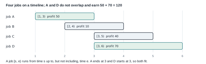
A job written [s, e) runs from time s up to, but not including, time e. So a job ending at 3 and a job
starting at 3 do not overlap.
6.4.1 Building the subproblem
First sort the jobs by end time. Then any job that can come before job i in a schedule ends earlier, so it appears earlier in the sorted list. The subproblem is:
dp[i]is the best profit using only the first i jobs of the sorted list.
For job i there are two choices:
- Skip it. The best profit stays
dp[i], the best without it. - Take it. Then only jobs that end by its start time can come before it. Those jobs are a prefix of the
sorted list, say the first
prevjobs. The profit isdp[prev] + profit of job i.
So dp[i + 1] is the larger of the two. The last entry is the answer.
Finding prev is a search in a sorted list, so it can be a binary search, like chapter 3’s. The standard
library provides one as partition_point. Given a condition that is true for a prefix of the list and false
after it, partition_point returns the length of that prefix.
6.4.2 The code
A job is a small Copy struct: when it starts, when it ends, and what it pays.
#[derive(Debug, Default, Clone, Copy)]
struct Job {
    start: u32,
    end: u32,
    profit: u64,
}
Listing 6.5 The complete program. src/bin/job_scheduling_with_profit_and_deadline.rs
#[derive(Debug, Default, Clone, Copy)]
struct Job {
    start: u32,
    end: u32,
    profit: u64,
}

fn max_profit(mut jobs: Vec<Job>) -> u64 {
    // Sort by end time so every job that could come before
    // job `i` in a schedule sits somewhere in jobs[..i].
    jobs.sort_unstable_by_key(|job| job.end);

    // dp[i] = best profit achievable using only the first `i` jobs.
    let mut dp = vec![0; jobs.len() + 1];

    for (i, job) in jobs.iter().enumerate() {
        // Binary search for how many earlier jobs finish by the time
        // this one starts. Those are exactly the jobs compatible with it,
        // and since they form a prefix, dp[prev] is their best profit.
        let prev = jobs[..i].partition_point(|j| j.end <= job.start);

        // Either skip this job (keep dp[i]),
        // or take it on top of the best compatible prefix.
        dp[i + 1] = dp[i].max(dp[prev] + job.profit);
    }

    // After considering every job, the last entry holds the answer.
    dp[jobs.len()]
}

fn main() {
    let jobs = vec![
        Job {
            start: 1,
            end: 3,
            profit: 50,
        },
        Job {
            start: 2,
            end: 4,
            profit: 10,
        },
        Job {
            start: 3,
            end: 5,
            profit: 40,
        },
        Job {
            start: 3,
            end: 6,
            profit: 70,
        },
    ];

    println!("{}", max_profit(jobs)); // 120
}
The comments inside max_profit walk through the same reasoning as section 6.4.1, step by step.
jobs[..i].partition_point(|j| j.end <= job.start) counts the jobs among the first i that end by this job’s
start. Because the list is sorted by end time, those jobs come first, which is the condition
partition_point needs.
Trace it on the sorted jobs A, B, C, D:
| i | job | prev | skip: dp[i] | take: dp[prev] + profit | dp[i + 1] |
|---|---|---|---|---|---|
| 0 | A [1, 3) 50 | 0 | 0 | 0 + 50 = 50 | 50 |
| 1 | B [2, 4) 10 | 0 | 50 | 0 + 10 = 10 | 50 |
| 2 | C [3, 5) 40 | 1 | 50 | 50 + 40 = 90 | 90 |
| 3 | D [3, 6) 70 | 1 | 90 | 50 + 70 = 120 | 120 |
For C and D, prev is 1: only A ends by time 3. Sorting costs O(n log n), and each job does one binary
search, so the whole program is O(n log n).
$ cargo run --bin job_scheduling_with_profit_and_deadline
120
6.5 Jobs that also need memory and cores
The problem. A cluster holds several GPUs. Each GPU has a fixed amount of memory and a fixed number of cores. Each job needs some of both, and it runs only on a GPU that has enough of each. A GPU runs one job at a time, as in section 6.4.
The program below answers a narrow question: which single GPU gives the best schedule? Section 6.5.4 measures what that leaves unused.
The sample cluster has two GPUs and the four jobs from section 6.4, with a memory need and a core need added.
| job | time | memory | cores | profit |
|---|---|---|---|---|
| A | [1, 3) | 12 GB | 20 | 50 |
| B | [2, 4) | 8 GB | 10 | 10 |
| C | [3, 5) | 40 GB | 60 | 40 |
| D | [3, 6) | 60 GB | 90 | 70 |
gpu 0 has 80 GB and 108 cores, so all four jobs fit there. Only A and B fit on gpu 1, which has 16 GB and 40 cores.
6.5.1 The fit test, and the same table
The new step is one boolean. A job fits a GPU when the GPU has at least its memory and at least its cores.
The rest is the table from section 6.4. Sort the jobs by end time and find each job’s compatible
prefix prev. Then fill dp with the better of skipping the job and taking it on top of dp[prev].
The fit test changes one line of that loop. A job that does not fit is skipped, as if it were not in
the list at all. Its entry in dp copies the entry before it.
6.5.2 The code
A job carries its two resource needs beside its time and its profit. A GPU carries the same two numbers, and one method answers whether a job fits.
#[derive(Debug, Default, Clone, Copy)]
struct Gpu {
    mem_gb: u32,
    cores: u32,
}

#[derive(Debug, Default, Clone, Copy)]
struct Job {
    start: u32,
    end: u32,
    mem_gb: u32,
    cores: u32,
    profit: u64,
}

impl Gpu {
    /// A job fits when the GPU has at least its memory and at least its cores.
    fn fits(&self, job: &Job) -> bool {
        (0..=self.mem_gb).contains(&job.mem_gb) && (0..=self.cores).contains(&job.cores)
    }
}
Listing 6.6 The complete program. src/bin/gpu_job_schedule.rs
//! Choose non-overlapping jobs for a GPU, where each job needs memory and cores.
//!
//! A job runs only on a GPU with enough memory and enough cores. For one GPU the
//! task is weighted interval scheduling: sort by end time, then take or skip each
//! job. The same table is reused for every GPU, and the best GPU wins.

#[derive(Debug, Default, Clone, Copy)]
struct Gpu {
    mem_gb: u32,
    cores: u32,
}

#[derive(Debug, Default, Clone, Copy)]
struct Job {
    start: u32,
    end: u32,
    mem_gb: u32,
    cores: u32,
    profit: u64,
}

impl Gpu {
    /// A job fits when the GPU has at least its memory and at least its cores.
    fn fits(&self, job: &Job) -> bool {
        (0..=self.mem_gb).contains(&job.mem_gb) && (0..=self.cores).contains(&job.cores)
    }
}

/// The best profit from work that runs on one GPU.
///
/// Every job it picks runs on the same GPU. That is the right model when a workload
/// is pinned to one device. Spreading the jobs over several GPUs is a different
/// problem, and the chapter measures what it is worth on the sample data.
fn max_profit(gpus: &[Gpu], mut jobs: Vec<Job>) -> u64 {
    jobs.sort_unstable_by_key(|job| job.end);

    // prev[i] = how many jobs finish by the time job `i` starts. The end times
    // are sorted, so each count is the length of a prefix, found in one search.
    let prev: Vec<usize> = jobs
        .iter()
        .map(|job| jobs.partition_point(|earlier| earlier.end <= job.start))
        .collect();

    // dp[i] = best profit using only the first `i` jobs. Reused for every GPU.
    let mut dp = vec![0; jobs.len() + 1];

    let pick_jobs_dp = |gpu: &Gpu| {
        for index in 0..jobs.len() {
            let job = &jobs[index];
            dp[index + 1] = if gpu.fits(job) {
                dp[index].max(dp[prev[index]] + job.profit)
            } else {
                dp[index]
            };
        }
        dp[jobs.len()]
    };

    gpus.iter()
        .map(pick_jobs_dp)
        .max()
        .unwrap_or(0)
}

#[cfg(test)]
mod tests {
    use super::*;

    fn large() -> Gpu {
        Gpu {
            mem_gb: 80,
            cores: 108,
        }
    }

    fn small() -> Gpu {
        Gpu {
            mem_gb: 16,
            cores: 40,
        }
    }

    fn sample_jobs() -> Vec<Job> {
        vec![
            Job {
                start: 1,
                end: 3,
                mem_gb: 12,
                cores: 20,
                profit: 50,
            },
            Job {
                start: 2,
                end: 4,
                mem_gb: 8,
                cores: 10,
                profit: 10,
            },
            Job {
                start: 3,
                end: 5,
                mem_gb: 40,
                cores: 60,
                profit: 40,
            },
            Job {
                start: 3,
                end: 6,
                mem_gb: 60,
                cores: 90,
                profit: 70,
            },
        ]
    }

    #[test]
    fn the_large_gpu_runs_the_best_pair() {
        assert_eq!(max_profit(&[large()], sample_jobs()), 120);
    }

    #[test]
    fn the_small_gpu_skips_what_does_not_fit() {
        assert_eq!(max_profit(&[small()], sample_jobs()), 50);
    }

    #[test]
    fn the_best_gpu_wins() {
        assert_eq!(max_profit(&[large(), small()], sample_jobs()), 120);
    }

    #[test]
    fn no_gpu_or_no_job_earns_nothing() {
        assert_eq!(max_profit(&[], sample_jobs()), 0);
        assert_eq!(max_profit(&[large()], Vec::new()), 0);
    }

    #[test]
    fn cores_alone_can_disqualify_a_job() {
        let jobs = vec![Job {
            start: 0,
            end: 1,
            mem_gb: 1,
            cores: 200,
            profit: 9,
        }];
        assert_eq!(max_profit(&[large()], jobs), 0);
    }
}

fn main() {
    let gpus = vec![
        Gpu {
            mem_gb: 80,
            cores: 108,
        },
        Gpu {
            mem_gb: 16,
            cores: 40,
        },
    ];

    let jobs = vec![
        Job {
            start: 1,
            end: 3,
            mem_gb: 12,
            cores: 20,
            profit: 50,
        },
        Job {
            start: 2,
            end: 4,
            mem_gb: 8,
            cores: 10,
            profit: 10,
        },
        Job {
            start: 3,
            end: 5,
            mem_gb: 40,
            cores: 60,
            profit: 40,
        },
        Job {
            start: 3,
            end: 6,
            mem_gb: 60,
            cores: 90,
            profit: 70,
        },
    ];

    println!("{}", max_profit(&gpus, jobs)); // 120
}
max_profit builds prev once and then reuses a single dp vector for each GPU. The closure
pick_jobs_dp fills the table for one GPU and returns its last entry. gpus.iter().map(pick_jobs_dp)
runs that closure for every GPU, and .max() keeps the best result.
Reusing dp is safe. The loop writes dp[i + 1] from dp[i] and dp[prev[i]]. Both indexes are at
most i, so it reads values this pass has already written. Every pass overwrites all of dp except
dp[0], which stays 0.
Animation 6.3 opens with the jobs out of order. It lifts them into end order, then shows each job’s arithmetic in a callout beside the table.
skip = dp[i] against take = dp[prev] + profit and writes max of the two into dp[i+1]. The fit test decides which jobs a GPU may take; the last part shares the jobs out for 130.6.5.3 Two tables
gpu 0 has enough of both for every job, so its table is the one from section 6.4.
| i | job | fits | prev | skip dp[i] | take dp[prev] + profit | dp[i+1] |
|---|---|---|---|---|---|---|
| 0 | A | yes | 0 | 0 | 0 + 50 = 50 | 50 |
| 1 | B | yes | 0 | 50 | 0 + 10 = 10 | 50 |
| 2 | C | yes | 1 | 50 | 50 + 40 = 90 | 90 |
| 3 | D | yes | 1 | 90 | 50 + 70 = 120 | 120 |
gpu 1 fails the fit test for C and D, so both are skipped and the table stops at 50.
| i | job | fits | prev | skip dp[i] | take | dp[i+1] |
|---|---|---|---|---|---|---|
| 0 | A | yes | 0 | 0 | 0 + 50 = 50 | 50 |
| 1 | B | yes | 0 | 50 | 0 + 10 = 10 | 50 |
| 2 | C | no | 1 | 50 | no fit | 50 |
| 3 | D | no | 1 | 50 | no fit | 50 |
The answer is max(120, 50) = 120.
$ cargo run --bin gpu_job_schedule
120
Sorting costs O(n log n), and each job finds its compatible prefix with one binary search. Each GPU
then fills its table in O(n), and the same dp is reused, so memory is O(n).
6.5.4 What one GPU at a time costs
max returns one GPU’s schedule. The other GPU runs nothing in that answer, even when it has room.
The two schedules cannot be added, because they overlap. The best schedule for gpu 1 is A alone, which earns 50. That A is already part of the 120 on gpu 0, so adding the two totals counts A twice.
Sharing the jobs out does better. Put A and D on gpu 0, and B on gpu 1. Neither GPU runs two overlapping jobs, and the total is 120 + 10 = 130.
Finding that split is a different problem. It has to decide which GPU runs each job. A table per GPU cannot express that choice, because the GPUs are not independent. With many jobs and many GPUs the search grows quickly, and production schedulers use heuristics, bin packing, or an integer program instead.
Summary
- Dynamic programming answers smaller versions of a problem first, saves the answers, and combines them.
- Start by writing, in one sentence, what one table entry means. The recurrence and the code follow from it.
- Coin change fills
dp[t]fromdp[t - c] + 1for each coin, left to right, in O(amount × coins). - Greedy choices can fail. Coins 1, 3, and 4 make 6 greedily with three coins, but two suffice.
- Backtracking explores a tree of choices with one shared
path, pushing before each recursive call and popping after it. Listing all subsets is O(n · 2ⁿ), the size of the output. - The longest increasing subsequence keeps the smallest possible ending for each length, in a sorted set, for O(n log n).
- Weighted job scheduling sorts by end time, uses
partition_pointto find compatible jobs, and fills a table of best profits. - A memory and a core need cost one boolean in that loop. A job that does not fit is skipped, and one
dpvector serves every GPU. - The best single GPU is not the same as the best use of all the GPUs. On the sample data, sharing the jobs out earns 130 where one GPU earns 120.
Chapter 7 begins Part 3, on modeling data. You will build types that can only hold valid values, using structs, enums, and error types.
Exercises
- Change
coin_changeto also return the coins it used. Store the last coin chosen for each amount, then follow those choices back fromamount. - Write the O(n²) version of the longest increasing subsequence described in section 6.3, and check that it
agrees with
lis_lenon random lists. - Generate all subsets without recursion. Count a number
maskfrom 0 to 2ⁿ − 1, and include element i when bit i ofmaskis set. - Extend
max_profitto return which jobs it chose, not only the total. - Change
max_profitso the jobs may be split across the GPUs. Work out the best total for the two GPUs and four jobs in section 6.5 by hand. Then explain why one table per GPU cannot find it.