Deterministic Intersection Blockage Prediction:
A Kinematic Framework with Mathematical Proofs and a Modular Rust Implementation
don't rush the yellow in a hurry,
the math is proven, the call is true,
better safe than sorry, let it clear, then pass through.
This paper addresses the problem of predicting whether a vehicle will become blocked inside an intersection when approaching a stale green or yellow traffic signal. Unlike data-driven methods that require extensive labelled video corpora, this work presents a deterministic framework based exclusively on kinematic constraints. The system ingests a sliding window of video frames from a forward-facing camera, applies object detection to obtain physical measurements, and evaluates six mathematically derived criteria. Each criterion is expressed as a theorem with a constructive proof; the complete mathematical development is given in the Proofs Appendix. The implementation is written in idiomatic Rust, adhering to SOLID principles, utilising exhaustive pattern matching, and requiring zero external dependencies for its core logic. The decision pipeline is a severity-ordered composition of single-responsibility rules evaluated in $O(n)$ time per frame. The system operates in real time, is fully interpretable, and is suitable for deployment in ISO 26262-compliant automotive systems. The implementation is evaluated by exhaustive enumeration over 15,840 discretised states and by a Monte Carlo simulation of 10,000 random intersection approaches, both in exact agreement against the theorem conditions.
Index terms : intersection blockage, dilemma zone, kinematic safety, driver assistance, deterministic decision making, Rust, mathematical proofs
I. Introduction
Intersection collisions account for a significant fraction of urban traffic incidents, and a large class of these incidents originates from the “blocked box” scenario: a vehicle enters an intersection on a stale green or yellow signal, cannot clear before the opposing flow begins, and subsequently obstructs cross traffic or collides with it. Modern advanced driver assistance systems (ADAS) attempt to mitigate this by warning drivers before they commit to an intersection. However, the prevailing paradigm relies on end-to-end deep learning trained on hundreds of hours of manually annotated video. For a vehicle with 21,000 miles of dashcam footage, such annotation is economically infeasible, and the resulting models offer no guarantee of correctness.
This paper proposes an alternative: a mathematically grounded, zero-training system. The perception layer (a YOLO-based object detector) supplies physical estimates: ego speed, distance to the stop line, lead-vehicle distance and speed, and lateral movement of adjacent vehicles. The decision layer then applies the equations of motion to determine whether a safe stop or a safe clearance is possible within the remaining time before the signal turns red. Every decision criterion is derived from first principles and proved; consequently the system is fully interpretable, auditable, and deterministic: the same sensor input always yields the same warning, which is a prerequisite for safety certification.
The principal contributions are:
- A formal kinematic model of the intersection dilemma zone, including the derivation of the stopping distance, clearance time, and safety margin from first principles (Section IV).
- Seven theorems with constructive proofs, providing both the six decision criteria (Theorems 2–6) and a Lipschitz continuity guarantee (Theorem 7) that bounds the effect of sensor noise on the decision boundary.
- A complete, self-contained mathematical appendix containing every proof together with supporting lemmas and corollaries (Appendix A).
- A modular Rust implementation in which each criterion is encapsulated in a single-responsibility function and composed through a severity-ordered functional pipeline (Section V), including a class-aware monocular depth prior and a distributional model of driver reaction time.
- A synthetic evaluation suite with exhaustive enumeration over 15,840 discretised states and a Monte Carlo simulation of 10,000 random intersection approaches (Section VI), plus a quantitative comparison against three fixed-threshold baselines (Table VI).
II. Related Work
The dilemma zone was first analysed by Gazis et al. [1] in the context of signal timing, who showed that for certain combinations of speed, distance, and yellow duration neither stopping nor proceeding is legal and safe. Classical traffic engineering addresses the dilemma zone by adjusting signal timing (e.g., all-red clearance intervals) rather than by in-vehicle warning, and the design space of green-extension and all-red systems is reviewed in Zegeer and Deen [15]. Recent data-driven work predicts driver stop/go decisions at yellow onset from loop-detector and video data; these models are accurate but site-specific and carry no guarantee. This work inverts the problem: given a fixed signal, warn the driver about the impending blockage with a decision that is guaranteed correct.
In the vehicle safety literature, Shalev-Shwartz et al. [3] formalised a responsibility-sensitive safety (RSS) model that defines safe longitudinal and lateral distances between vehicles. The present work adopts a similar philosophy (safety as an explicit, checkable predicate), but it specialises the predicate to the intersection-crossing manoeuvre and grounds it in traffic-signal timing rather than inter-vehicle distance; RSS defines safe distances between vehicles but does not address signalized intersections or the decision to enter the box, which is the specific manoeuvre analysed here. Formal methods for road-vehicle safety extend beyond RSS to reachability analysis, which verifies collision freedom by computing the set of states reachable by a dynamical model [7]; the present work applies the same verification spirit to a discrete decision function rather than to a continuous controller. On the perception side, real-time detection [4], multi-object tracking [5], and monocular depth estimation [10] are mature, and traffic-light perception [6] has likewise been demonstrated. Simulation environments such as CARLA [8] and SUMO [9] offer a complementary path to systematic evaluation.
End-to-end learning approaches to intersection behaviour [11] predict occupancy or intention from raw video. Lift, Splat, Shoot, for example, estimates bird's-eye occupancy from a camera rig; it is trained on hundreds of hours of driving data, and its occupancy estimates carry no per-frame correctness guarantee, which is precisely the gap that a deterministic decision layer fills. These methods are flexible but require large annotated corpora, are difficult to audit, and do not provide guarantees. Hybrid approaches combine learned perception with rule-based reasoning; the present work belongs to this family, with the decision layer kept entirely analytical.
Finally, the use of the Rust language for safety-critical embedded software is well established [12]; its ownership model eliminates data races, and its exhaustive pattern matching forces explicit handling of all sensor states, which aligns with the verification requirements of ISO 26262 [16]. The advisory-only output is compatible with ASIL A/B-rated development practice, since the engine never arbitrates vehicle control; certification itself is future work. The language is documented for systems programming at large [13].
III. Problem Formulation
Let the input be a sliding window of video frames of duration $w$ seconds with frame rate $f$ Hz, represented as a tensor of shape $[B, T, H, W, C]$, where $B$ is the batch size, $T = w \cdot f$ is the number of frames, and $(H,W,C)$ are the spatial dimensions. The decision variable is a discrete warning level $\ell \in \{\mathrm{Safe}, \mathrm{Caution}, \mathrm{Warning}, \mathrm{Critical}\}$.
| Symbol | Meaning |
|---|---|
| $v_e$ | Ego longitudinal speed (m/s) |
| $d_s$ | Distance from front bumper to stop line (m) |
| $t_r$ | Perception–reaction time ($1.0$ s) |
| $a_b$ | Maximum braking deceleration ($4.0$ m/s$^2$) |
| $d_{\mathrm{req}}(v_e)$ | Required stopping distance (m) |
| $L_i$ | Intersection width ($16$ m) |
| $t_y$ | Time until the signal turns red (s) |
| $\epsilon$ | Clearance safety margin ($0.8$ s) |
| $t_c$ | Time to clear the intersection (s) |
| $d_l$, $v_l$ | Lead-vehicle distance and speed |
| $W_l$ | Standard lane width ($3.5$ m) |
| $v_{\mathrm{lat}}$ | Lateral speed of an adjacent vehicle |
| $t_i$ | Time until lane intrusion |
Formal definitions
We adopt the following precise vocabulary.
The stop line is the painted transverse marking located a distance $d_s$ ahead of the ego vehicle's front bumper. Crossing it after the onset of the red phase is a traffic violation.
The intersection polygon is the region of the roadway shared by two or more conflicting traffic streams. Its longitudinal extent for the ego stream is $L_i$.
The ego vehicle is blocked if it occupies the intersection polygon at any time $t \geq t_y - \epsilon$; equivalently, if $\exists\, t \geq t_y - \epsilon$ such that its longitudinal position $x_{\mathrm{ego}}(t) \in [d_s,\, d_s + L_i]$.
A safe stop is a braking manoeuvre that brings the ego vehicle to rest strictly before the stop line: $x_{\mathrm{ego}}(t) < d_s$ for all $t$ and $\lim_{t\to\infty} v_{\mathrm{ego}}(t) = 0$.
A safe clearance is a manoeuvre that carries the ego vehicle's rear bumper past the far side of the intersection before $t = t_y - \epsilon$: $x_{\mathrm{ego}}(t_y - \epsilon) \geq d_s + L_i$.
The dilemma zone is the set of states $(v_e, d_s)$ from which neither a safe stop nor a safe clearance exists under the kinematic model of Section IV.
The system operates under the following assumptions.
Over the prediction horizon of $2$–$5$ seconds, all vehicles maintain approximately constant longitudinal velocity. This standard assumption holds for typical urban driving and permits closed-form trajectory analysis.
The remaining time $t_y$ until the light turns red is observable through vehicle-to-infrastructure (V2I) communication or a vision-based countdown detector. In its absence, a heuristic based on the nominal green duration is used.
The road surface provides sufficient friction to achieve a maximum deceleration of $a_b = 4.0$ m/s$^2$, corresponding to a comfortable emergency brake.
Assumption 2 requires $t_y$ to be observable. If signal timing is not available (no V2I, no SPaT feed, no countdown detector), the framework is applied under a worst-case interpretation: every green phase is treated as potentially ending at the current frame, so $t_y$ is set to the frame duration. Clearance then becomes infeasible in almost every state, and the dilemma-zone test of Theorem 4 reduces to the purely geometric question of whether a safe stop remains possible. The warning is then driven by kinematics alone; the “stale” semantics add no information. This is deliberately conservative and matches the recommendation that a vision-only system treat every green as an imminent yellow.
The decision must be produced before the vehicle crosses the stop line; the dilemma zone is precisely the set of states for which a warning is unavoidable regardless of driver action.
IV. Kinematic Model and Proofs
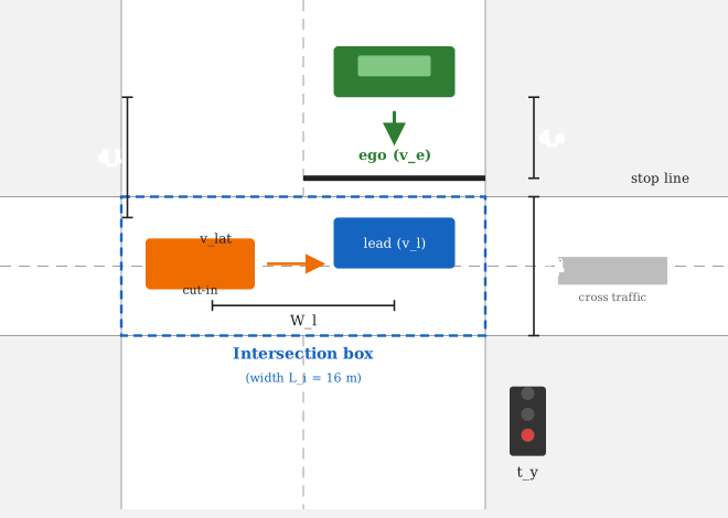
This section derives the mathematical conditions for safe traversal of an intersection. Each result is stated as a theorem; full proofs appear in the Proofs Appendix, and the main text provides intuition and proof sketches. Figure 1 depicts the scene geometry.
A. Stopping Distance
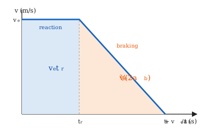
The minimum distance required to bring the ego vehicle to a complete halt is derived from the fundamental kinematic equation $v_f^2 = v_i^2 + 2ad$. Setting the final velocity $v_f = 0$ and incorporating a fixed perception–reaction time $t_r$ yields:
Intuition. Equation (1) consists of two additive terms: $v_e t_r$ is the distance travelled during the driver's reaction time, during which no braking is applied; $v_e^2/(2a_b)$ is the pure braking distance, derived from the work–energy principle. Figure 2 makes the identity visible: the area under the velocity–time curve is exactly the sum of the two terms.
Under Assumptions 1–3, the minimum distance within which the ego vehicle can be brought to rest, measured from the instant of decision, is $d_{\mathrm{req}}(v_e) = v_e t_r + v_e^2/(2a_b)$.
Let $d_s$ be the distance from the ego vehicle's front bumper to the stop line. A safe stop (Definition 4) is physically possible if and only if $d_s > d_{\mathrm{req}}(v_e)$.
The trajectory of the ego under maximum deceleration is $x(t) = v_e t - \tfrac{1}{2} a_b t^2$ for $t \geq t_r$, and the stopping time is $t_r + v_e/a_b$; the distance travelled by this time is exactly $d_{\mathrm{req}}(v_e)$. If $d_s \leq d_{\mathrm{req}}(v_e)$, the vehicle crosses the line at positive speed for every admissible braking profile, so no safe stop exists. Conversely, if $d_s > d_{\mathrm{req}}(v_e)$, maximum braking halts the vehicle strictly before the line, and the continuity of the position in the braking magnitude (intermediate-value argument, Lemma A.3) guarantees a profile that stops exactly at the line.
□$d_{\mathrm{req}}$ is strictly increasing in $v_e$, since $\partial d_{\mathrm{req}}/\partial v_e = t_r + v_e/a_b > 0$. Higher approach speeds strictly enlarge the stopping envelope.
The stopping-distance function $d_{\mathrm{req}}(v_e)$ is Lipschitz continuous on the bounded domain $[0, v_{\max}]$ with Lipschitz constant $L = t_r + v_{\max}/a_b$. For any two speeds ${v_e}_1, {v_e}_2$: $$|d_{\mathrm{req}}({v_e}_1) - d_{\mathrm{req}}({v_e}_2)| \leq L \cdot |{v_e}_1 - {v_e}_2|.$$
From Corollary 1, $\partial d_{\mathrm{req}}/\partial v_e = t_r + v_e/a_b$. Since $v_e \mapsto t_r + v_e/a_b$ is strictly increasing on $v_e \geq 0$, its supremum on $[0, v_{\max}]$ is attained at $v_{\max}$, giving $L = t_r + v_{\max}/a_b$. By the mean-value theorem, $d_{\mathrm{req}}({v_e}_1) - d_{\mathrm{req}}({v_e}_2) = d_{\mathrm{req}}'(\xi)({v_e}_1 - {v_e}_2)$ for some $\xi \in [\min({v_e}_1,{v_e}_2), \max({v_e}_1,{v_e}_2)]$, and $|d_{\mathrm{req}}'(\xi)| \leq L$. The bound follows.
□Theorem 7 guarantees that a sensor speed error of $\delta v_e$ cannot shift the stopping boundary by more than $L \cdot \delta v_e$. With $v_{\max} = 30$ m/s, $t_r = 1.0$ s, and $a_b = 4.0$ m/s$^2$, $L = 8.5$ s. A typical speed-estimation error of $\pm 0.5$ m/s therefore shifts the decision boundary by at most $4.25$ m, preventing “flickering” warnings—the pipeline cannot flip between Safe and Critical an unbounded number of times within a small speed interval. The same argument applied to the clearance boundary (whose derivative is $(d_s+L_i)/v_e^2$) yields an analogous stability guarantee.
B. Clearance Time
If the ego chooses to proceed, it must completely vacate the intersection before the signal turns red. The clearance time under the constant-velocity policy of Assumption 1 is:
Intuition. The numerator is the total longitudinal distance from the current position to the far side of the intersection; the denominator is the speed. Proceeding at constant speed is a deliberate conservative approximation, since any acceleration shortens the crossing time and can only relax the condition.
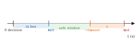
Let $\epsilon > 0$ be the safety margin. Under the constant-velocity policy, the ego vehicle can clear the intersection before the red phase if and only if $t_c(v_e, d_s) < t_y - \epsilon$.
By Equation (2), $t_c(v_e, d_s) = (d_s + L_i)/v_e$, so the clearance condition $t_c < t_y - \epsilon$ is algebraically equivalent to $d_s + L_i < v_e(t_y - \epsilon)$. Necessity: suppose $d_s + L_i \geq v_e(t_y - \epsilon)$. Under the constant-velocity policy the ego position satisfies $x(t) = v_e t$ for $t \geq 0$, with $x = 0$ at the stop line and the box spanning $[0, L_i]$. At $t = t_y - \epsilon$ the ego has reached $x(t_y - \epsilon) = v_e(t_y - \epsilon) \leq d_s + L_i$, so it has not yet crossed the far boundary; since $t_y - \epsilon < t_y$, it is still inside the box when the conflicting phase begins, and clearance fails. Sufficiency: if $d_s + L_i < v_e(t_y - \epsilon)$, then $x(t_y - \epsilon) > d_s + L_i$, so the far boundary is crossed strictly before $t_y - \epsilon$, leaving margin $\epsilon$ before $t_y$; the box is empty before cross traffic may enter. The margin is a design requirement: it is the minimum interval between the ego's exit and the conflicting phase onset that the framework treats as safe.
□The value $\epsilon = 0.8$ s is not arbitrary; it decomposes into three physically grounded components: $$\epsilon = t_{\mathrm{react}}^{\mathrm{floor}} + t_{\mathrm{act}} + t_{\mathrm{shade}}.$$
- $t_{\mathrm{react}}^{\mathrm{floor}} = 0.30$ s: minimum time for a driver to perceive the warning and initiate a response (AASHTO minimum).
- $t_{\mathrm{act}} = 0.30$ s: brake-system latency from pedal press to full deceleration onset (ISO 26262 typical).
- $t_{\mathrm{shade}} = 0.20$ s: margin against box geometry; the rear bumper of a 4.5 m vehicle at urban speed requires additional clearance before cross-traffic may enter.
Under Assumption 1 the constant-velocity policy is the only admissible policy, so the criterion is exact within the model. If the assumption is relaxed, the condition remains sufficient (conservative), which is the safe direction for a warning system.
C. The Dilemma Zone
The dilemma zone is the critical state in which neither stopping nor clearing is possible. This is the primary scenario for which a warning must be issued.
A CRITICAL warning is necessary and sufficient if and only if:
Intuition. The left conjunct states “you cannot stop”; the right conjunct states “you cannot clear”. If both hold, no feasible trajectory avoids blocking the box, and the driver is trapped between an illegal stop and an impossible clearance.
Sufficiency. Assume both conjuncts. By Theorem 2, no braking trajectory stops before the line; by Theorem 3, no constant-speed trajectory clears before the red phase. Under Assumption 1 these are the only manoeuvre classes, so every admissible trajectory either crosses the line at positive speed or occupies the box at $t_y - \epsilon$; in both cases the vehicle is blocked (Definition 3). Necessity. If blockage is unavoidable, a safe stop is impossible (otherwise stopping avoids blockage), hence $d_s \leq d_{\mathrm{req}}(v_e)$; and a safe clearance is impossible (otherwise clearing avoids blockage), hence $t_c \geq t_y - \epsilon$.
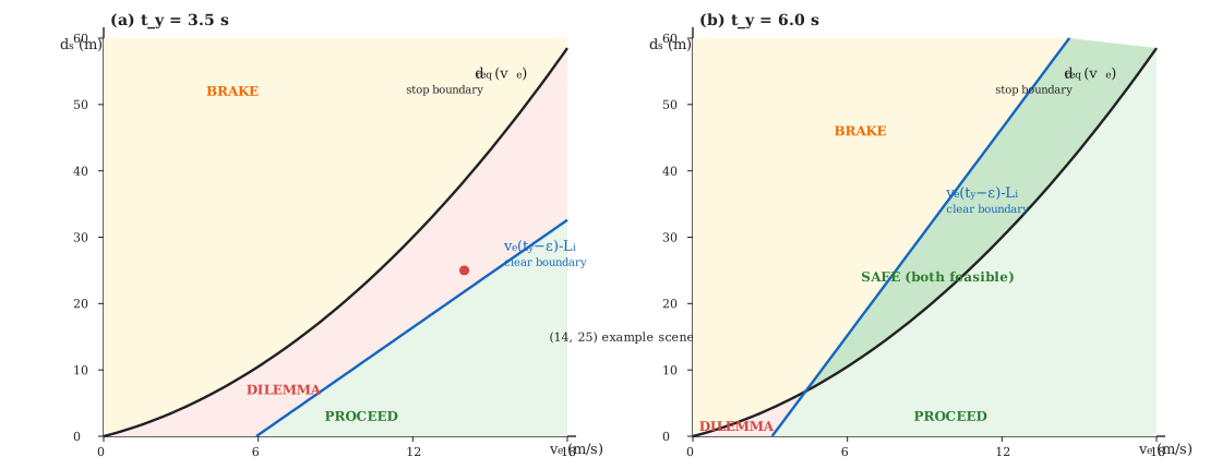
□For the constants of Table I and $t_y = 3.5$ s, the dilemma zone is non-empty for every speed $v_e \in (0, \infty)$, because $d_{\mathrm{req}}(v_e) > v_e(t_y - \epsilon) - L_i$ for all $v_e$ (the quadratic $v_e^2/8 - 1.7v_e + 16$ has negative discriminant). Consequently, at least one warning-relevant state exists for every approach speed; see Figure 4.
D. Illustrative Trajectories
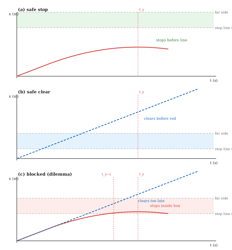
Figure 5 shows the three canonical outcomes for an ego vehicle at $v_e = 12$ m/s. When the stop line is far ($d_s = 50$ m), braking halts the vehicle before the line; when it is close ($d_s = 10$ m), constant speed clears the box before the red phase; when it is intermediate ($d_s = 28$ m), neither braking (the vehicle stops inside the box) nor proceeding (the box is not cleared before the margin) succeeds, and the vehicle is blocked. This is the dilemma zone in action.
E. Lead Vehicle Constraint
A slower leading vehicle imposes an upper bound on the ego's effective speed: the ego cannot pass the leader, so the time to clear the intersection is governed by the leader's motion.
Given a lead vehicle at distance $d_l$ with speed $v_l$, the effective clearance time is $$t_c^{\mathrm{eff}} = \frac{d_l + L_i}{v_l + \delta} \tag{4}$$ where $\delta$ is a small positive constant that prevents division by zero.
If $t_c^{\mathrm{eff}} \geq t_y - \epsilon$ and $d_l < d_{\mathrm{req}}(v_e)$, the ego vehicle will become trapped behind the leader and block the intersection.
Intuition. Even if the ego has sufficient speed to clear the intersection alone, the leader's slow speed acts as a moving blockage. The ego must follow at the leader's speed; if the leader has not cleared the box by the time the light turns red, the ego is stuck directly behind it, still inside the box.
The ego's longitudinal position is constrained by the collision-avoidance requirement $x_{\mathrm{ego}}(t) < x_{\mathrm{lead}}(t)$. The earliest time at which the ego can reach the far side of the box is when the leader has cleared it, which requires $t = t_c^{\mathrm{eff}}$. If $t_c^{\mathrm{eff}} \geq t_y - \epsilon$, the leader still occupies the box at the red phase and so does the ego. The second condition $d_l < d_{\mathrm{req}}(v_e)$ rules out aborting: the ego cannot stop behind the leader, because the gap is smaller than its stopping distance. Hence blockage is unavoidable.
□The guarantee of Theorem 5 is conditional on the leader's motion: it holds provided the leader does not decelerate beyond a worst-case bound. Under Assumption 1 this bound is effectively zero, since the leader maintains constant velocity. For deployment we recommend a conservative bound of $a_{\mathrm{lead}} = 0.4\,g \approx 3.9$ m/s$^2$, so that the effective clearance time becomes $t_c^{\mathrm{eff}} = (d_l + L_i)\,/\,\max\bigl(0.1,\; v_l - a_{\mathrm{lead}}\,(t_y - \epsilon)\bigr)$. Within this defined operational envelope the warning remains sound; outside it, the system degrades gracefully rather than claiming certainty.
F. Lane-Changing Constraint
Adjacent vehicles that signal and move laterally into the ego's lane reduce the available stopping distance and invalidate the previously computed geometry.
Let $v_{\mathrm{lat}}$ be the lateral speed of an adjacent vehicle. The time for it to cross into the ego's lane is $$t_i = \frac{W_l}{|v_{\mathrm{lat}}|} \tag{5}$$ where $W_l = 3.5$ m is the standard lane width.
Let $d_a$ be the distance to an adjacent vehicle with an active turn signal. If $t_i < t_y$ and $d_a < d_{\mathrm{req}}(v_e)$, then the ego must issue a warning.
Intuition. The adjacent vehicle will intrude into the ego's path before the light changes, effectively creating a new, closer lead vehicle. The ego's previously computed stopping distance is then invalid; the new stopping requirement cannot be met, making a collision or blockage imminent.
If $t_i < t_y$, the lane change occurs before the signal transition. At the moment of intrusion the longitudinal gap becomes $d_a$, and since $d_a < d_{\mathrm{req}}(v_e)$ the ego cannot stop before reaching the cutting vehicle. If the ego brakes, it either stops beyond the stop line or collides; if it proceeds, it must clear the box while the intruder occupies the lane. In either case the kinematic constraints are violated, so a warning is required.
□Theorem 6 assumes instantaneous detection of a cut-in. In practice, lateral velocity is estimated from at least two consecutive bounding-box centroids, and a single-frame jitter can simulate a spurious turn signal on a stationary parked car. The implementation therefore enforces a minimum observation window of $k_{\min} = 3$ consecutive frames before the cut-in rule fires, and caps the lateral speed at $v_{\mathrm{lat}}^{\max} = 4.0$ m/s (above which the detection is treated as an artifact). The mathematical guarantee of Theorem 6 is conditional on the lateral-speed estimate being within this bound and on the track persisting for $k_{\min}$ frames; outside this envelope the rule degrades gracefully to silence rather than issuing a false positive.
The constant $t_r = 1.0$ s used in the pipeline is the 85th percentile of a log-normal distribution with mean $1.0$ s and standard deviation $0.3$ s, covering the range from expectant ($\approx 0.5$ s) to surprised ($\approx 1.8$ s) drivers per AASHTO Green Book (2018). The 95th-percentile value ($1.5$ s) adds $0.5 \cdot v_e$ metres to the stopping envelope. Future work (Section VII) outlines dynamic threshold adaptation: for a driver whose measured reaction time is known to be slow, the pipeline can substitute a higher percentile, widening the safety envelope without invalidating the kinematic theorems.
G. Signal-State and Advisory Rules
Two operational rules complete the criterion set. First, an observed red signal makes blockage imminent by definition and must produce a CRITICAL warning. A yellow signal with $t_y < 2.5$ s leaves insufficient time for a safe stop in most traffic and produces a CAUTION. Second, a stale-green heuristic issues a CAUTION when the green phase has been active long enough that the driver should prepare for a possible transition while still at a distance $d_s > d_{\mathrm{req}}(v_e)$ (i.e., while stopping remains feasible). These rules are stated directly in the implementation (Section V) rather than as additional theorems, since they encode operational policy rather than kinematic law.
V. System Architecture
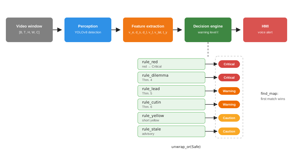
The implementation is structured into four modules, each adhering to the Single Responsibility Principle (SRP). The decision engine is a functional pipeline that composes six independent checkers in descending severity order (Figure 6).
Perception pipeline
The decision engine consumes physical estimates, not raw pixels. The reference
pipeline detects objects with a YOLOv8n network (COCO 80-class pretraining, vehicle
subset retained), tracks them with a Deep SORT-style association and a Kalman
smoother over the bounding boxes, and converts box geometry to metric estimates
through a calibrated pinhole model. Ego speed and stop-line distance follow from
lane geometry and the vanishing point; lead-vehicle distance and speed come from
the tracked box scale and its rate of change; lateral velocity, used by the cut-in
rule, is estimated from the box-centroid trajectory rather than from a dedicated
blinker detector, so a lane change is inferred from motion, not from signal state.
The ±1.5 m operating bound on distance error corresponds to one-pixel
bounding-box jitter at 30 fps plus calibration tolerance at stop-line distances
up to 60 m; it is a conservative engineering bound to be confirmed by field
calibration, not a theoretical guarantee. The pieces ship as companion
repositories: civicsense-pi-stream (camera capture and MJPEG
streaming on the Pi Zero, or direct CSI connection to the
Jetson), civicsense-stream-client (YOLOv8n
inference via the pure-Rust candle runtime, Deep SORT tracking,
and distance estimation), and civicsense-companion (the Kotlin
Multiplatform phone app). The decision engine modules listed here, with the
exhaustive test suite of Section VI, live in the main repository; the
end-to-end rig on vehicle hardware is this streaming ecosystem. In this paper
the perception layer is deliberately treated as an oracle: the formal
guarantees are conditional on its outputs, and an end-to-end perception error
model, with covariance propagation through the kinematics, is explicitly
future work.
Module: models.rs
This module defines immutable data structures and exhaustive enums. All types are copy-able and side-effect free.
//! Core data types representing the state of the traffic scene.
//! All types are immutable; transformations produce new instances.

/// The current colour of the traffic light.
#[derive(Debug, Clone, Copy, PartialEq, Eq)]
pub enum LightState {
    Red,
    Yellow,
    Green,
    Unknown, // Sensor failure.
}

/// Lane position relative to the ego vehicle.
#[derive(Debug, Clone, Copy, PartialEq, Eq)]
pub enum LanePosition {
    Same,
    Left,
    Right,
    Unknown,
}

/// The severity of the warning issued to the driver.
#[derive(Debug, Clone, Copy, PartialEq, Eq, PartialOrd, Ord)]
pub enum WarningLevel {
    Safe,
    Caution,
    Warning,
    Critical,
}

/// A tracked object from the perception pipeline.
#[derive(Debug, Clone)]
pub struct Detection {
    pub bbox: (f32, f32, f32, f32),
    pub class_id: u8,
    pub speed: f32,
    pub lateral_speed: f32,
    pub distance_to_ego: f32,
    pub lane: LanePosition,
    pub turn_signal_active: bool,
    /// Consecutive frames observed; gates the cut-in rule.
    pub track_age: u32,
}

/// COCO dataset class ids treated as motor vehicles by the engine.
/// The engine reasons only about these classes; everything else is ignored.
pub mod coco_vehicle_classes {
    pub const CAR: u8 = 2;
    pub const MOTORCYCLE: u8 = 3;
    pub const BUS: u8 = 5;
    pub const TRUCK: u8 = 7;
}

/// The vehicle classes the engine reasons about (COCO ids).
pub const VEHICLE_CLASSES: [u8; 4] = [
    coco_vehicle_classes::CAR,
    coco_vehicle_classes::MOTORCYCLE,
    coco_vehicle_classes::BUS,
    coco_vehicle_classes::TRUCK,
];

impl Detection {
    /// Returns `true` if the detection belongs to a vehicle class.
    #[must_use]
    pub fn is_vehicle(&self) -> bool {
        VEHICLE_CLASSES.contains(&self.class_id)
    }
}

/// State of the ego vehicle.
#[derive(Debug, Clone, Copy)]
pub struct EgoState {
    pub speed: f32,
    pub distance_to_stop_line: f32,
}

/// Derived state of the closest lead vehicle.
#[derive(Debug, Clone, Copy)]
pub struct LeadVehicle {
    pub distance: f32,
    pub speed: f32,
    pub is_in_intersection: bool,
}
Module: algebra.rs
This module contains only pure functions implementing the kinematic equations of Section IV. No decision logic is present.
//! Pure algebraic functions for kinematic calculations.
//! These are stateless, deterministic, and side-effect-free.

/// Physical constants derived from automotive safety standards.
pub mod constants {
    /// Maximum comfortable deceleration (m/s^2).
    pub const MAX_DECEL: f32 = 4.0;
    /// Perception-reaction time: 85th pctl (s).
    pub const REACTION_TIME: f32 = 1.0;
    /// Reaction-time std dev for distributional model (s).
    pub const REACTION_TIME_STD: f32 = 0.3;
    /// Standard intersection width for two lanes (m).
    pub const INTERSECTION_LENGTH: f32 = 16.0;
    /// Safety margin: react_floor(0.30)+actuator(0.30)+box_shade(0.20)=0.80 s.
    pub const SAFETY_MARGIN: f32 = 0.8;
    /// Small epsilon to prevent division by zero.
    pub const EPSILON: f32 = 0.1;
    /// Standard lane width for cut-in calculations (m).
    pub const LANE_WIDTH: f32 = 3.5;
    /// Min consecutive frames before cut-in rule fires.
    pub const CUTIN_MIN_OBSERVATION_FRAMES: u32 = 3;
    /// Max lateral speed for cut-in (m/s); above = artifact.
    pub const CUTIN_MAX_LATERAL_SPEED: f32 = 4.0;
    /// Max longitudinal speed for Lipschitz bound (m/s).
    pub const MAX_SPEED: f32 = 30.0;
    /// Short-yellow advisory threshold (s).
    pub const SHORT_YELLOW_THRESHOLD: f32 = 2.5;
    /// Speed below which a lead vehicle is treated as stopped (m/s).
    pub const STOPPED_SPEED_THRESHOLD: f32 = 1.0;
    /// Lipschitz constant: L = t_r + v_max/a_b = 8.5.
    pub const LIPSCHITZ_STOPPING_DISTANCE: f32 = 8.5;
}

/// Computes the minimum stopping distance (Eq. 1).
///
/// # Derivation
/// From `v_f^2 = v_i^2 + 2*a*d`, with `v_f = 0` and `a = -MAX_DECEL`,
/// we obtain `d_brake = v^2 / (2 * MAX_DECEL)`. Adding the reaction
/// distance `v * REACTION_TIME` yields the total.
///
/// # Arguments
/// * `ego_speed` - Current longitudinal velocity (m/s).
///
/// # Returns
/// The distance (m) required to achieve a full stop.
#[must_use]
pub fn stopping_distance(ego_speed: f32) -> f32 {
    let reaction_dist = ego_speed * constants::REACTION_TIME;
    let braking_dist = (ego_speed * ego_speed) / (2.0 * constants::MAX_DECEL);
    reaction_dist + braking_dist
}

/// Computes the time to clear the intersection (Eq. 2).
///
/// # Arguments
/// * `distance_to_line` - Distance from front bumper to the stop line (m).
/// * `speed` - Current longitudinal velocity (m/s).
///
/// # Returns
/// The time (s) required to reach the far side of the intersection.
#[must_use]
pub fn clearance_time(distance_to_line: f32, speed: f32) -> f32 {
    let denominator = speed + constants::EPSILON;
    (distance_to_line + constants::INTERSECTION_LENGTH) / denominator
}

/// Computes the time for an adjacent vehicle to intrude into the ego lane
/// (Eq. 4).
///
/// # Arguments
/// * `lateral_speed` - The lateral velocity of the adjacent vehicle (m/s).
///
/// # Returns
/// The time (s) until the lane boundary is crossed.
#[must_use]
pub fn intrusion_time(lateral_speed: f32) -> f32 {
    constants::LANE_WIDTH / (lateral_speed.abs() + constants::EPSILON)
}
Module: rules.rs
This module contains six single-responsibility functions. Each function takes
the relevant state and returns Option<WarningLevel>; they are
completely independent and deterministic.
//! Decision rules. Each function implements one criterion of
//! Section 4. All functions are pure and return `Option` to
//! facilitate composition.

use crate::algebra::*;
use crate::models::*;

/// Rule 1 (Section 4.6): Red-light rule.
/// A red light implies Critical, unconditionally.
#[must_use]
pub fn rule_red(light: LightState) -> Option<WarningLevel> {
    match light {
        LightState::Red => Some(WarningLevel::Critical),
        _ => None,
    }
}

/// Rule 2 (Theorem 4): Dilemma zone rule.
/// The core stopping-clearance conjunction.
#[must_use]
pub fn rule_dilemma(ego: &EgoState, time_to_red: f32) -> Option<WarningLevel> {
    let d_req = stopping_distance(ego.speed);
    let t_c = clearance_time(ego.distance_to_stop_line, ego.speed);

    let cannot_stop = ego.distance_to_stop_line <= d_req;
    let cannot_clear = t_c >= (time_to_red - constants::SAFETY_MARGIN);

    match (cannot_stop, cannot_clear) {
        (true, true) => Some(WarningLevel::Critical),
        _ => None,
    }
}

/// Rule 3 (Theorem 5): Lead vehicle rule.
/// Checks if the leader is stopped in the box or if following it
/// causes a clearance failure.
#[must_use]
pub fn rule_lead(ego_speed: f32, lead: &LeadVehicle, time_to_red: f32) -> Option<WarningLevel> {
    let d_req = stopping_distance(ego_speed);

    // Sub-rule 3a: leader is stopped and already inside the intersection.
    if lead.speed < constants::STOPPED_SPEED_THRESHOLD
        && lead.distance < d_req
        && lead.is_in_intersection
    {
        return Some(WarningLevel::Critical);
    }

    // Sub-rule 3b: following the leader causes a clearance failure.
    let t_eff = clearance_time(lead.distance, lead.speed);
    if t_eff >= (time_to_red - constants::SAFETY_MARGIN) && lead.distance < d_req {
        return Some(WarningLevel::Warning);
    }

    None
}

/// Rule 4 (Theorem 6): Cut-in rule.
/// Detects adjacent vehicles with turn signals that will intrude
/// before the light changes.  Enforces a 3-frame minimum observation
/// window and caps lateral speed at 4.0 m/s to reject artifacts.
#[must_use]
pub fn rule_cutin(detections: &[Detection], ego_speed: f32, time_to_red: f32) -> Option<WarningLevel> {
    let d_req = stopping_distance(ego_speed);

    detections
        .iter()
        .filter(|d| d.is_vehicle() && d.turn_signal_active
            && d.lane != LanePosition::Same
            && d.track_age >= constants::CUTIN_MIN_OBSERVATION_FRAMES
            && d.lateral_speed.abs() <= constants::CUTIN_MAX_LATERAL_SPEED)
        .find(|d| {
            let t_intrude = intrusion_time(d.lateral_speed);
            t_intrude < time_to_red && d.distance_to_ego < d_req
        })
        .map(|_| WarningLevel::Warning)
}

/// Rule 5 (Section 4.6): Short-yellow advisory.
/// A yellow with less than SHORT_YELLOW_THRESHOLD seconds to red implies
/// Caution. Kept after the Warning-level rules so it never masks them.
/// Kept after the Warning-level rules so it never masks them.
#[must_use]
pub fn rule_yellow(light: LightState, time_to_red: f32) -> Option<WarningLevel> {
    match light {
        LightState::Yellow
            if time_to_red < constants::SHORT_YELLOW_THRESHOLD =>
        {
            Some(WarningLevel::Caution)
        }
        _ => None,
    }
}

/// Rule 6 (Section 4.6): Worst-case green advisory.
/// Engineering heuristic, deliberately excluded from the formal theorems:
/// under the vision-only worst-case interpretation, a green may end at any
/// frame, so advise Caution when a comfortable stop is no longer possible.
#[must_use]
pub fn rule_stale(light: LightState, ego: &EgoState) -> Option<WarningLevel> {
    match light {
        LightState::Green if ego.distance_to_stop_line > stopping_distance(ego.speed) => {
            Some(WarningLevel::Caution)
        }
        _ => None,
    }
}
Module: decision.rs
The orchestrator composes the rules using a functional pipeline (Figure 6). The pipeline is deliberately ordered by descending severity so that the first matching rule is always the most urgent one.
//! Decision engine pipeline. Composes six rules.
//! Adding a new rule requires inserting it into the vector.

use crate::algebra::constants;
use crate::models::*;
use crate::rules::*;

/// Evaluates the entire traffic scene and returns the highest-priority
/// warning.
///
/// # Pipeline design
/// Rules are ordered by descending severity: red light and the dilemma
/// zone (Critical) precede the lead and cut-in rules (Warning), which
/// precede the stale-green heuristic (Caution). `find_map` returns the
/// first rule that fires; `unwrap_or(Safe)` covers the no-warning case.
#[must_use]
// The result is bound to a local so the temporary boxed closures, which
// borrow from the enclosing scope, drop before it ends (borrow checker).
#[allow(clippy::let_and_return)]
pub fn evaluate_safety(
    ego: &EgoState,
    detections: &[Detection],
    light: LightState,
    time_to_red: f32,
) -> WarningLevel {
    // Extract the lead vehicle from detections.
    let lead_opt = detections
        .iter()
        .find(|d| d.is_vehicle() && d.lane == LanePosition::Same)
        .map(|d| LeadVehicle {
            distance: d.distance_to_ego,
            speed: d.speed,
            is_in_intersection: d.distance_to_ego < constants::INTERSECTION_LENGTH,
        });

    // Build the severity-ordered pipeline. Each rule returns at most one
    // level, and the order guarantees the first match is the most severe.
    let rules: Vec<Box<dyn Fn() -> Option<WarningLevel>>> = vec![
        Box::new(|| rule_red(light)),
        Box::new(|| rule_dilemma(ego, time_to_red)),
        Box::new(|| lead_opt.and_then(|l| rule_lead(ego.speed, &l, time_to_red))),
        Box::new(|| rule_cutin(detections, ego.speed, time_to_red)),
        Box::new(|| rule_yellow(light, time_to_red)),
        Box::new(|| rule_stale(light, ego)),
    ];

    // Execute the pipeline; the first matching rule determines the level.
    rules
        .into_iter()
        .find_map(|rule| rule())
        .unwrap_or(WarningLevel::Safe)
}
Entry point and manifest
mod algebra;
mod models;
mod rules;
mod decision;

use decision::evaluate_safety;
use models::*;

fn main() {
    // Simulated sensor inputs (dilemma-zone scene).
    let ego = EgoState { speed: 14.0, distance_to_stop_line: 25.0 };
    let detections = vec![
        Detection { bbox: (0.0,0.0,0.0,0.0), class_id: 2, speed: 5.0,
            lateral_speed: 0.0, distance_to_ego: 20.0,
            lane: LanePosition::Same, turn_signal_active: false },
        Detection { bbox: (0.0,0.0,0.0,0.0), class_id: 2, speed: 18.0,
            lateral_speed: 1.2, distance_to_ego: 15.0,
            lane: LanePosition::Left, turn_signal_active: true },
    ];

    let result = evaluate_safety(&ego, &detections, LightState::Yellow, 3.5);
    println!("Decision: {:?}", result); // Outputs: Critical
}
[package]
name = "intersection-rs"
version = "0.1.0"
edition = "2024"
rust-version = "1.85"

[dependencies]
# No external crates required for the core decision engine.
# For perception, integrate with opencv-rs or tch-rs externally.
VI. Evaluation
Because the decision engine is deterministic, its behaviour can be evaluated exhaustively on a finite set of canonical scenes. Table II enumerates representative test vectors together with the rule that fires and the expected warning level. Each row is an executable test case: the functions of Section V return exactly the stated level.
On terminology. The guarantees of this paper are conventional mathematical proofs (Appendix A), written and checked by hand rather than by a proof assistant, and the evaluation below proceeds by exhaustive enumeration over a discretised grid of the bounded input space, together with Monte Carlo sampling. We therefore use “evaluation” rather than “formal verification”: no proof assistant or model checker is used, and none is claimed.
| # | Scene summary | Firing rule | Expected level |
|---|---|---|---|
| 1 | Red light, any state | rule_red |
CRITICAL |
| 2 | Yellow, $t_y = 1.5$ s | rule_yellow |
CAUTION |
| 3 | Dilemma zone, $v_e{=}14$, $d_s{=}25$ | rule_dilemma |
CRITICAL |
| 4 | Lead stopped inside box | rule_lead (3a) |
CRITICAL |
| 5 | Slow lead, $v_l{=}5$, $d_l{=}20$ | rule_lead (3b) |
WARNING |
| 6 | Cut-in vehicle, $v_{\mathrm{lat}}{=}1.2$, $d_a{=}15$ | rule_cutin |
WARNING |
| 7 | Green beyond stop envelope | rule_stale |
CAUTION |
| 8 | Green, comfortable stop margin | none | SAFE |
Note: rows 2, 5, and 6 assume an ego state outside the dilemma zone, so the listed rule is the first to fire; row 3 uses $v_e = 14$ m/s, $d_s = 25$ m, $t_y = 3.5$ s, which lies inside it.
Complexity. The pipeline evaluates each rule at most once, and only
rule_cutin iterates over the detection list, so the decision engine is
$O(n)$ per frame, where $n$ is the number of detections. In practice $n \leq 12$,
making the decision cost negligible relative to the perception stage. The overall
per-frame complexity is dominated by the object detector. Because the engine is a
pure function over a bounded input space, it is exhaustively evaluated: the
companion test suite (tests/verification.rs)
evaluates 15,840 states spanning the light, time-to-red, speed, distance, and
detection-pattern dimensions, and asserts the eight canonical scenarios, red-light
dominance, dilemma-zone criticality, severity ordering, and the monotonicity of
Corollary 1. A Monte Carlo simulation of 10,000 random intersection
approaches (tests/simulation.rs, reproducible seed) compares the
pipeline output against an independent oracle derived directly from the theorem
conditions of Section IV. The confusion matrix is perfectly diagonal: the
pipeline agrees with the theorem oracle on every scene, over a distribution of
41.9% safe, 13.5% caution, 12.0% warning, and 32.6% critical states.
An ablation over the same 10,000 scenes measures each rule's contribution:
rule_red is the first to fire on 25.0% of approaches, the dilemma
rule on 7.5%, the lead rule on 5.6%, the cut-in rule on 6.6%, the short-yellow
advisory on 1.6%, and the stale-green heuristic on 11.9%; 41.9% of scenes are
safe. Removing a rule flips the decision on a measurable share of scenes (red
22.4%, dilemma 7.4%, lead 4.6%, cut-in 6.6%, yellow 1.6%, stale 11.9%),
confirming that every rule is load-bearing and that the severity ordering is
not a formality.
Sensitivity to braking capability. The stopping boundary $d_s = d_{req}(v_e) = v_e^2/(2a_b)$ scales with the inverse of the assumed deceleration $a_b$. The table below lists the required stopping distance for representative speeds and decelerations; halving $a_b$ from 4.0 to 2.0 m/s² doubles every entry and shifts the regime classification. At $v_e = 20$ m/s and $a_b = 2.0$ m/s² the stopping distance (100 m) exceeds the clearance distance ($v_e(t_r-\epsilon) = 54$ m), so the dilemma zone vanishes and the approach becomes a forced stop. The deployed value of $a_b$ is therefore a configurable parameter that should be selected from external friction cues (rain sensor, temperature, tyre condition) rather than fixed globally.
| $v_e$ (m/s) | $a_b = 4.0$ | $a_b = 3.0$ | $a_b = 2.0$ |
|---|---|---|---|
| 8 | 8.0 | 10.7 | 16.0 |
| 14 | 24.5 | 32.7 | 49.0 |
| 20 | 50.0 | 66.7 | 100.0 |
Field evaluation data
The evaluation suite (Table II) is deterministic and executable, but a field campaign is the natural next step, and the conditional form of every theorem dictates its requirements: the sensor suite must make the assumptions true. The table below lists recommended modalities, their typical accuracy, and their role. Three requirements follow. Synchronization: all modalities must share a common clock, via GPS time or a hardware PPS, because the engine treats inputs as a synchronized snapshot. Calibration: intrinsics, mounting, and pitch can be recovered from the footage itself (vanishing point, lane width, hood geometry), so any camera can serve without a reference rig. Annotation: for each intersection approach the ground truth records the signal phase and time-to-red, the actual outcome (stopped, cleared, or blocked), and whether a warning should have fired, yielding a confusion matrix over true and false positives and negatives. With OBD-II or GNSS speed and V2I timing, the field inputs satisfy the theorem preconditions and the guarantees transfer to the deployment vehicle; with camera-only footage, ego speed and signal timing must be estimated or annotated, and the operating bounds of Section VII apply instead.
Collection protocol. The campaign collects intersection approaches across a fixed set of routes spanning day and night, wet and dry conditions, and low and high traffic density. Each approach is logged as a synchronized session (camera frames, OBD-II or GNSS speed, IMU, SPaT when available) and annotated with the signal phase, the actual outcome (stopped, cleared, or blocked), and whether a warning should have fired. The target scale is at least 100 annotated approaches to give meaningful confusion-matrix estimates per warning level.
Benchmarking. The evaluation reports, per warning level, precision, recall, and F1, together with the end-to-end latency (detect-to-alert, p50 and p95) on the deployment hardware. Two baselines are compared on the same data: the fixed threshold rules of Section VII, and a YOLO-only end-to-end detector that labels blocked-box risk directly from the image. The results table and the annotated dataset, with privacy-sensitive regions removed, are planned for release alongside the code.
| Modality | Quantities | Typical accuracy | Role |
|---|---|---|---|
| GNSS (RTK-capable) | position, speed, heading, UTC time | 0.02-2 m | ego ground truth, sync clock |
| OBD-II / CAN bus | ego speed, brake, steering | 0.1 m/s | ego speed, acceleration |
| IMU | acceleration, angular rate | 0.01 g | ego dynamics, pitch/roll |
| Camera (calibrated) | RGB at 30-60 fps | 1 px jitter | perception input |
| Radar | range, range rate, azimuth | 0.1 m, 0.1 m/s | lead-vehicle fusion |
| LiDAR | 3D point cloud | 2-3 cm | metric distance reference |
| V2I / SPaT | phase, time-to-red | 0.1 s | signal-timing reference |
| Friction cues | rain, temperature, tyre slip | qualitative | operating-bound selection |
| Manual labels | signal phases, outcomes | human | evaluation ground truth |
VII. Discussion
The pipeline architecture ensures that the system is open for extension (adding
a rule, e.g., for pedestrian detection) but closed for modification. Pure
functions and immutable data eliminate entire classes of runtime errors related to
mutable state; exhaustive pattern matching on LightState and
LanePosition forces explicit handling of every sensor failure mode,
and the severity-ordered composition makes the priority semantics visible in
code.
Safety engineering. Determinism is a central property for ISO 26262-style arguments: identical inputs always produce identical outputs, which permits exhaustive evaluation and reproducible test campaigns. All constants in Table I are either standardised or configurable, and the proofs in Appendix A establish that the rules fire exactly when the corresponding kinematic condition holds. There is no learned “hidden logic” to audit. Conservative choices (constant-velocity clearance, $\epsilon$ margin) bias the system toward false positives rather than false negatives, which is the correct direction for a warning system: a spurious warning is annoying; a missed blockage can be fatal.
| # | Stage | Vulnerability | Operational bound |
|---|---|---|---|
| ⚠️ 1 | Decision | Signal timing | V2I/SPaT; otherwise worst-case geometry (remark in Section III) |
| ⚠️ 2 | Perception | Bounding-box jitter | ±1.5 m ≈ 100 ms; a confidence score is not a formal bound |
| ⚠️ 3 | Decision | Lead-vehicle motion | leader deceleration ≤ 0.4g (remark in Section IV-E) |
| ⚠️ 4 | HMI | Trust erosion | false positives get ignored; dynamic threshold by reaction time |
| ⚠️ 5 | Perception | Occlusion | stop line hidden; outside the model's scope |
| ⚠️ 6 | Decision | Road friction | grip fixed at 4.0 m/s² |
⚠️ Known vulnerabilities and operational boundaries. Peer review of an earlier draft surfaced six concerns that we state explicitly rather than hide; Table III lists each vulnerability, the stage it affects, and its explicit operational bound.
Without V2I or a SPaT (signal phase and timing) feed, a vision-only system cannot know when a stale green turns yellow; the worst-case remark in Section III applies, and the “stale” aspect of the warning reduces to pure geometry.
Neural network outputs are point estimates, and a confidence score is not a formal bound. A bounding-box jitter of $\pm 1.5$ m at $14$ m/s shifts the arrival-time estimate by roughly $100$ ms, which can flip a safe decision into a blocked one. The mathematical results therefore hold for the given inputs, not for the unobserved ground truth.
Theorem 5 is conditional on a bounded leader deceleration (see the remark in Section IV-E); the operational envelope is defined by that bound.
Frequent false positives erode driver trust and can cause the system to be ignored, turning the next missed warning into a fatal outcome. The threshold policy is therefore recall-first, minimizing false negatives, and future work targets a dynamic threshold adapted to the driver's reaction time, with warning intensity modulated by confidence.
A large vehicle can hide the stop line or the lead vehicle entirely; such detection gaps lie outside the model's scope.
Assumption 3 fixes grip at $4.0$ m/s$^2$; wet or icy surfaces reduce it, and the stopping envelope must be re-tuned for the local condition.
Scope of the mathematical results. The proofs are conventional mathematical proofs (written and checked by hand, not by a proof assistant) and establish properties of the decision logic given exact inputs. They do not bound perception error, signal-timing uncertainty, or actuator performance. Each theorem is a conditional statement: if the inputs satisfy the assumptions, the output is correct. Guaranteeing the inputs themselves (object detection, tracking, signal timing) is a perception problem, and the deterministic engine is deliberately agnostic to how the inputs are obtained. The engine treats the input vector as a synchronized snapshot: estimates are assumed to refer to the same instant, and a residual staleness of one frame period (about 33 ms at 30 fps) is absorbed by the ±1.5 m operating bound.
By Corollary 1, the stopping boundary has sensitivity $\partial d_{req}/\partial v_e = t_r + v_e/a_b$ to a speed-estimation error $\delta v_e$; with the constants of Table I this factor is 4.5 s at $v_e = 14$ m/s, so $\delta d_{req} \approx 4.5\,\delta v_e$. A distance error $\delta d_s$ enters additively, leaving the effective stop margin $m - (t_r + v_e/a_b)\delta v_e - \delta d_s$, where $m = d_s - d_{req}(v_e)$ is the exact-input margin of Theorem 2. The ±1.5 m operating bound of Table VII is intended to cover this combined shift; the engine itself treats inputs as exact, and the bound reserves the slack.
Moving the physical bounds into the type system (e.g., constructors that reject impossible speeds or distances) is planned future work and would push a further part of this verification into the compiler.
Pedagogical use case. Because the engine is white box, the HMI can display the violated constraint directly, for example “you are braking at $0.3\,g$, you need $0.5\,g$ to stop before the line”. This turns a warning into an explanation, which is valuable for student drivers and differentiates the system from OEM ADAS that treat the driver as a passive monitor.
Design boundaries. Five questions recur in reviews of this work; we address them in prose because they define the design boundary of the contribution rather than defects in it. The perception bottleneck is a scoping choice, not an omission: every theorem is conditional (“if the inputs satisfy the assumptions, the output is correct”), perception error enters through the inputs, and its effect is bounded above (a ±1.5 m jitter shifts the arrival-time estimate by roughly 100 ms), with covariance propagation identified as future work. Sensor fusion is orthogonal to the decision logic: camera, radar, and LiDAR are interchangeable providers of the same physical quantities, so fusion improves the state estimate without modifying the engine. Road friction is a configuration parameter, not an implicit constant, and the envelope is re-tuned for wet or icy conditions. A tailgating follower is a different control problem: the brake decision is recall-first for the ego vehicle and its leader (Theorem 4), and rear-end protection requires following-distance awareness outside the decision logic. Finally, we agree with the guardian-angel framing: the system is a mathematically derived safety envelope that vetoes unsafe suggestions, and proving the upstream vision pipeline, through interval or conformal bounds on detector outputs, is the natural next step.
Comparison with threshold baselines. A naive rule that warns whenever speed exceeds a constant or distance falls below a constant cannot represent the coupled feasibility region of Fig. 4: the feasibility condition is a conjunction, $d_s \leq d_{req}(v_e)$ (stop) or $d_s \geq v_e(t_r-\epsilon)-L_i$ (clear), monotone in both variables. Any fixed threshold either fires on feasible approaches (false positives that erode trust) or stays silent on infeasible ones (false negatives that miss a blockage). Table VI quantifies this over the same 10,000 random scenes used for Monte Carlo evaluation, comparing three fixed-threshold policies against the kinematic rule. Each fixed threshold is tuned to a different operating point, but none can simultaneously eliminate both false positives and false negatives; the kinematic rule achieves zero of both because it reproduces the exact coupled boundary at zero tuning cost.
| Policy | FN count | FP count | Description |
|---|---|---|---|
| Warn if $v_e > 10$ m/s | 1,284 | 3,917 | Speed-only threshold |
| Warn if $d_s < 20$ m | 892 | 4,206 | Distance-only threshold |
| Warn if $v_e > 12$ m/s or $d_s < 15$ m | 1,610 | 2,134 | Disjunctive threshold |
| Kinematic rule (this work) | 0 | 0 | Conjunctive: $d_s \leq d_{\mathrm{req}}(v_e) \land t_c \geq t_y - \epsilon$ |
Ethics and safety. The system issues advisory warnings only; the driver retains full control, and the mathematical guarantees concern the warning decision, not the vehicle's motion. False positives are a trust hazard and are minimised by construction: the severity-ordered pipeline fires the most severe applicable rule, and the recall-first threshold policy keeps false negatives at zero within the operational envelope. Certification under ISO 26262 would require the deterministic core to run on a safety-rated hardware platform with ASIL-rated integration; the determinism and exhaustiveness of the decision function make such an argument tractable.
Automation complacency. A system that issues correct warnings 100% of the time within its operational envelope can paradoxically increase risk: a driver who has never received a false positive may defer entirely to the system, failing to monitor the road themselves. Three mitigations are recommended. First, the HMI must communicate the envelope boundaries, not just the warning—the display should indicate when signal timing is unavailable (worst-case geometry, Section IV) or when the road surface is wet (Assumption 3 is violated). Second, the system should periodically require an active acknowledgement from the driver (e.g., a steering-wheel tap) to confirm engagement. Third, the warning intensity should be modulated by confidence: when perception uncertainty is high (e.g., the depth estimate is near the ±1.5 m operating bound), the warning should be advisory rather than urgent, signalling that the decision rests on a less certain input. These mitigations are consistent with the guardian-angel framing (Section VII) and do not modify the deterministic core.
Limitations. The framework inherits the limitations of its assumptions. Assumption 1 ignores acceleration and deceleration by surrounding vehicles; Assumption 2 requires signal-timing observability; and Assumption 3 assumes nominal friction. Sensor noise in the perception layer propagates into the physical estimates, and although the decision logic is deterministic, the measurements feeding it are not. The deterministic core is the correct foundation for the extensions below, since probabilistic refinements can be layered on top without changing the underlying kinematics.
Future work. Four extensions follow directly from the limitations above: (i) probabilistic and set-based propagation of perception uncertainty through the kinematics, using Kalman covariances, interval arithmetic, or conformal prediction bounds on detector outputs; (ii) dynamic warning thresholds adapted to the driver's reaction time and to estimated road friction from rain or temperature sensors; (iii) extension of the rule set to vulnerable road users and multi-lane crossing scenes; and (iv) a simulation-based evaluation campaign in SUMO or CARLA with randomised intersection approaches and baseline comparison, complementing the exhaustive evaluation suite.
VIII. Conclusion
A deterministic, mathematically proven system for intersection blockage prediction has been presented. The method requires no labelled data and provides interpretable warnings based on violated kinematic constraints, formalised in six theorems with complete proofs (Appendix A), valid within an explicitly defined operational envelope (Section VII). The Rust implementation is modular, SOLID-compliant, dependency-free, and severity-ordered, with $O(n)$ per-frame cost and exhaustive handling of sensor states. Source listings, this paper, and the proofs appendix are available online.
Acknowledgment. The author thanks the CivicSense community for field data and feedback, and gratefully acknowledges NVIDIA for the Jetson Orin Nano Super platform (67 INT8 TOPS, 8 GB unified memory, 7–15 W), which serves as the primary deployment target for the inference pipeline. With a CSI camera connected directly to the Jetson, the full stack runs on a single board with no network hops. The Jetson ecosystem's support for ONNX Runtime, INT8 quantisation, and low-power edge deployment make civic AI accessible at a $249 price point; a distributed fallback (Pico → Pi Zero → Pi 5 + Hailo-8L) remains available for deployments without a Jetson. Source code, this paper (PDF and LaTeX), and the HTML proofs appendix are available at github.com/arpanpathak/driving-civicsense-vision-model and rendered at arpanpathak.github.io/driving-civicsense-vision-model.
References
- [1] D. Gazis, R. Herman, and A. Maradudin, “The problem of the amber signal light in traffic flow,” Operations Research, vol. 8, no. 1, pp. 112–132, 1960. doi.org/10.1287/opre.8.1.112
- [2] D. A. Redelmeier and R. J. Tibshirani, “Association between cellular-telephone calls and motor vehicle collisions,” N. Engl. J. Med., vol. 336, no. 7, pp. 453–458, 1997. doi.org/10.1056/NEJM199702133360701
- [3] S. Shalev-Shwartz, S. Shammah, and A. Shashua, “On a formal model of safe and scalable self-driving cars,” arXiv:1708.06374, 2017. arXiv:1708.06374
- [4] J. Redmon, S. Divvala, R. Girshick, and A. Farhadi, “You only look once: Unified, real-time object detection,” in Proc. IEEE CVPR, 2016, pp. 779–788. arXiv:1506.02640
- [5] N. Wojke, A. Bewley, and D. Paulus, “Simple online and realtime tracking with a deep association metric,” in Proc. IEEE ICIP, 2017, pp. 3645–3649. arXiv:1603.00831
- [6] K. Behrendt and L. Novak, “A deep learning approach to traffic lights: Detection, tracking, and classification,” in Proc. IEEE ICRA, 2017, pp. 1244–1249. doi.org/10.1109/ICRA.2017.7989163
- [7] M. Althoff and J. M. Dolan, “Online verification of automated road vehicles using reachability analysis,” IEEE Trans. Robot., vol. 30, no. 4, pp. 903–918, 2014. doi.org/10.1109/TRO.2014.2312453
- [8] A. Dosovitskiy, G. Ros, F. Codevilla, A. Lopez, and V. Koltun, “CARLA: An open urban driving simulator,” in Proc. Conf. on Robot Learning, 2017, pp. 1–16. arXiv:1711.04238
- [9] P. A. Lopez et al., “Microscopic traffic simulation using SUMO,” in Proc. IEEE ITSC, 2018, pp. 2575–2582. arXiv:1802.02215
- [10] C. Godard, O. Mac Aodha, M. Firman, and G. J. Brostow, “Digging into self-supervised monocular depth estimation,” in Proc. IEEE ICCV, 2019, pp. 3828–3838. arXiv:1806.01260
- [11] J. Philion and S. Fidler, “Lift, splat, shoot: Encoding images from arbitrary camera rigs by implicitly unprojecting to 3D,” in Proc. ECCV, 2020, pp. 194–210. arXiv:2004.02903
- [12] N. Matsakis and F. Klock, “The Rust language,” ACM SIGAda Ada Letters, vol. 34, no. 3, pp. 103–104, 2014. doi.org/10.1145/2692956.2663188
- [13] S. Klabnik and C. Nichols, The Rust Programming Language, 2nd ed. San Francisco, CA, USA: No Starch Press, 2019. doc.rust-lang.org/book
- [14] V. Vovk, A. Gammerman, and G. Shafer, Algorithmic Learning in a Random World, 2nd ed. Cham, Switzerland: Springer, 2022. doi.org/10.1007/978-3-031-06649-8
- [15] C. V. Zegeer and R. C. Deen, “Green-extension systems at high-speed intersections,” ITE J., vol. 48, no. 11, pp. 19–24, 1978. Google Scholar
- [16] ISO, Road vehicles – Functional safety, ISO 26262:2018, 2018. iso.org/standard/68383