Chapter 19: Stencils and Jacobi Iteration
The temperature inside a heated plate, the electric potential between charged conductors and the pressure of a fluid at rest are all described by the same partial differential equation, the Laplace equation. A computer solves this equation on a grid of points. The value at each point is computed again and again from the values of its 4 neighbors, until the values stop changing. A computation in which every point of a grid is updated from a fixed pattern of neighbors is called a stencil computation. Stencils are among the most common workloads of a GPU, because all points of a grid can be updated at the same time.
In this chapter, we derive the parallel algorithm for 1 stencil, the 5-point stencil of the Laplace equation, together with its standard solver, Jacobi iteration. We work on a single 6 × 6 plate from the first section to the last. We first compute its steps by hand and show why an update in place produces a different answer. We then prove that 2 buffers used in turn compute Jacobi iteration exactly, and we count the memory traffic that determines the speed of the kernel. Both implementations, in Rust and in CUDA C++, check themselves against the values that we work out by hand.
This chapter covers
- the Laplace equation on a grid, and the 5-point stencil derived from it
- Jacobi iteration, worked by hand on a 6 × 6 plate
- why an update in place computes a different method, and the exact wrong value it produces
- Two buffers used in turn, and a proof that they compute Jacobi iteration
- One thread per cell, in Rust with
DisjointSliceand in C++ with__restrict__ - how fast the iteration converges, measured and predicted
- arithmetic intensity, and why a stencil is limited by memory bandwidth
The code of the chapter is in
code/oxide/ch19_stencil/
for Rust and in
code/cuda/ch19_stencil/
for C++.
19.1 The problem
19.1.1 A heated plate
We use the same example throughout the chapter. It is a square plate whose 4 edges are held at fixed temperatures, the top edge at 100 degrees and the other 3 edges at 0 degrees. Heat flows into the plate through the hot edge and out of it through the cold ones. After enough time, the temperature at every point stops changing, and we want to know this final temperature at every point of the plate.
A computer cannot store a temperature for each of the infinitely many points of the plate, so we replace the plate by a grid of 6 × 6 cells and keep 1 temperature per cell. The rows and the columns are numbered from 0 to 5, as shown in Figure 19.1. The cells on the edge of the grid have known temperatures, and the 16 cells inside them are the unknowns that we want to compute.
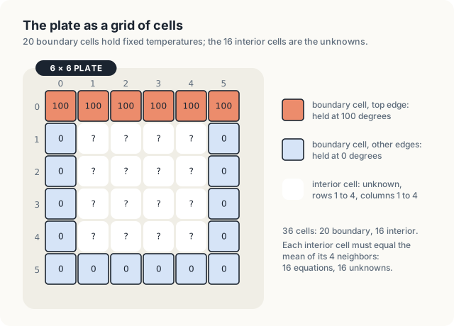
Definition 19.1 Grid, boundary cell, interior cell. A grid of \(W \times H\) cells holds one value per cell; cell \((r, c)\) lies in row \(r \in [0, H)\) and column \(c \in [0, W)\). A boundary cell lies in the first or last row or column; its value is given by the problem and never changes. Every other cell is an interior cell, and its value is unknown.
Example. Our plate has \(W = H = 6\): 36 cells, of which 20 are boundary cells and \(4 \times 4 = 16\) are interior cells, in rows 1 to 4 and columns 1 to 4.
Here \(W\) is the width of the grid, that is, the number of cells in a row, and \(H\) is its height, the number of cells in a column. As in the earlier chapters, \([a, b)\) denotes the integers from \(a\) to \(b - 1\), so \(r \in [0, 6)\) means that the row number \(r\) is one of 0, 1, 2, 3, 4 and 5.
The grid is stored in row-major order: the 6 cells of row 0 come first, followed by the 6 cells of row 1, then those of row 2, until row 5 ends the array. Before cell \((r, c)\) there are \(r\) complete rows of \(W\) cells each, followed by \(c\) cells of its own row, so cell \((r, c)\) is element \(rW + c\) of the array. For example, cell (2, 3) of our plate is element \(2 \cdot 6 + 3 = 15\). It follows that the 2 neighbors of a cell in the same row are 1 element away from it, at elements 14 and 16 in this example, while the 2 neighbors in the same column are \(W\) elements away, at elements \(15 - 6 = 9\) and \(15 + 6 = 21\).
19.1.2 The rule for the final temperature
Physics gives a simple rule that the final temperatures obey. At every interior cell, the temperature is the mean of the temperatures of its 4 neighbors:
\[ u_{r,c} = \frac{1}{4} \left( u_{r-1,c} + u_{r+1,c} + u_{r,c-1} + u_{r,c+1} \right). \]
| Symbol | Meaning | In the example, cell (1, 1) |
|---|---|---|
| \(u_{r,c}\) | final temperature of the cell in row \(r\), column \(c\) | \(u_{1,1} = 45.45\) |
| \(u_{r-1,c}\), \(u_{r+1,c}\) | temperatures of the cells above and below | 100 and 22.35 |
| \(u_{r,c-1}\), \(u_{r,c+1}\) | temperatures of the cells to the left and right | 0 and 59.47 |
| \(\frac{1}{4}\) | weight of each neighbor; 4 weights of 1/4 form a mean | 0.25 |
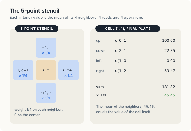
The reason for the rule is that heat flows from warm to cold. If a cell were warmer than the mean of its neighbors, it would lose more heat to them than it receives, and its temperature would still be falling. If it were colder, it would still be rising. Only when every cell equals the mean of its neighbors does the temperature stop changing. We can check the rule on the answer. In Section 19.2, we compute the final temperatures of our plate, and there cell (1, 1) holds 45.45, while its neighbors hold 100 above, 22.35 below, 0 to the left and 59.47 to the right. Their mean is \((100 + 22.35 + 0 + 59.47) / 4 = 181.82 / 4 = 45.45\), which is the value of the cell itself, as Figure 19.2 shows.
The rule is the discrete form of the Laplace equation. Let \(u(x, y)\) denote the temperature at the point \((x, y)\) of the plate. The Laplace equation states that the sum of the second derivatives of \(u\) along \(x\) and along \(y\) is 0 at every point inside the plate:
\[ \frac{\partial^2 u}{\partial x^2} + \frac{\partial^2 u}{\partial y^2} = 0. \]
| Symbol | Meaning | On the grid |
|---|---|---|
| \(u(x, y)\) | temperature at the point \((x, y)\) | \(u_{r,c}\), with \(x\) along the columns and \(y\) along the rows |
| \(\partial^2 u / \partial x^2\) | second derivative of \(u\) along \(x\): how fast the slope changes from left to right | a difference of the cells left and right |
| \(\partial^2 u / \partial y^2\) | the same along \(y\), from top to bottom | a difference of the cells above and below |
A grid has no derivatives, only values at cells, so we approximate each second derivative by a difference of neighboring values. Let \(h\) be the spacing between the centers of 2 neighboring cells. The second derivative along \(x\) at cell \((r, c)\) is approximated by the finite difference
\[ \frac{\partial^2 u}{\partial x^2} \approx \frac{u_{r,c+1} - 2u_{r,c} + u_{r,c-1}}{h^2}, \]
and the second derivative along \(y\) by the same expression with the cells above and below. The numerator compares the cell with its 2 neighbors in the row. It is 0 when the 3 values lie on a straight line, and it measures how far they bend away from one when they do not. We can test the approximation on a function whose second derivative we know. For \(f(x) = x^2\), whose second derivative is 2 everywhere, the difference at \(x = 1\) with \(h = 1\) uses \(f(2) = 4\), \(f(1) = 1\) and \(f(0) = 0\), and gives \((4 - 2 \cdot 1 + 0) / 1^2 = 2\), which is exact.
Substituting both differences into the Laplace equation gives
\[ \frac{u_{r,c+1} - 2u_{r,c} + u_{r,c-1}}{h^2} + \frac{u_{r+1,c} - 2u_{r,c} + u_{r-1,c}}{h^2} = 0. \]
Multiplying by \(h^2\) removes the spacing, and moving the 4 terms \(-2u_{r,c}\) to the right gives \(u_{r-1,c} + u_{r+1,c} + u_{r,c-1} + u_{r,c+1} = 4u_{r,c}\). Dividing by 4 gives the rule above. Note that the spacing \(h\) has canceled, so the rule is the same however finely we cut the plate.
Definition 19.2 Stencil. A stencil is a fixed pattern of neighbors, with a weight for each, from which a new value of a cell is computed. A stencil computation applies the same stencil to every interior cell of a grid. The 5-point stencil uses a cell and its 4 neighbors in the same row and column, with weight 1/4 on each neighbor and 0 on the cell itself.
Example. Applied to cell (1, 1) of the final plate, the 5-point stencil gives 45.45 (Figure 19.2).
The rule gives 1 equation for each of the 16 interior cells, and each equation contains up to 4 unknowns. For cell (1, 1), whose upper and left neighbors are boundary cells with the known values 100 and 0, the equation reads \(u_{1,1} = (100 + u_{2,1} + 0 + u_{1,2}) / 4\). A system of 16 equations can be solved by elimination, as in a first course in linear algebra. A grid of 4096 × 4096 cells, however, has 16.7 million interior cells, and elimination on a system of that size needs far more memory and time than the iterative method of the next section.
Exercises
19.1 Write the equation of the rule for cell (2, 3) of the plate. Which of its neighbors are
boundary cells?
19.2 At which element of the array is cell (4, 1) stored, in row-major order with \(W = 6\)?
19.3 Apply the finite difference to \(f(x) = x^3\) at \(x = 1\) with \(h = 1\) and with
\(h = 0.5\), and compare both with the exact second derivative, 6.
19.2 The sequential algorithm
19.2.1 Jacobi iteration
We do not know the final temperatures, but we do know a property that they have. Each interior value is the mean of its neighbors. Jacobi iteration turns this property into a procedure. It starts from a guess and replaces every interior value by the mean of its neighbors, again and again. If the guess is wrong, the replacement moves each value toward the mean of its neighbors, and after many repetitions the values settle at the point where the replacement no longer changes them, which is exactly the final state.
Definition 19.3 Jacobi iteration. Let \(u^{(0)}\) be a grid whose boundary cells hold the given values and whose interior cells hold a guess. Jacobi iteration computes the grids \(u^{(1)}, u^{(2)}, \ldots\), where each step keeps the boundary cells and sets every interior cell to
\[ u^{(k+1)}_{r,c} = \frac{1}{4} \left( u^{(k)}_{r-1,c} + u^{(k)}_{r+1,c} + u^{(k)}_{r,c-1} + u^{(k)}_{r,c+1} \right). \]
The right-hand side uses only values of step \(k\).
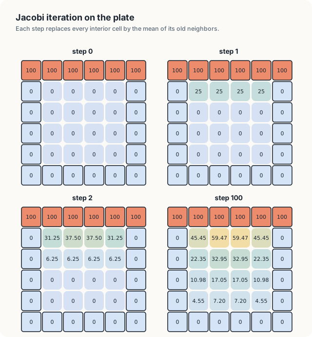
Example. We start from 0 in every interior cell. After step 1, the 4 cells of row 1 hold 25; all other interior cells still hold 0.
The superscript in parentheses is the number of the step, not a power. Thus \(u^{(0)}\) is the starting grid, \(u^{(1)}\) the grid after 1 step, and \(u^{(k)}_{r,c}\) the value of cell \((r, c)\) after \(k\) steps.
| Symbol | Meaning | In the example |
|---|---|---|
| \(k\) | number of steps already performed | \(k = 0\) when step 1 is computed |
| \(u^{(k)}\) | grid after \(k\) steps; the old grid that the step reads | \(u^{(0)}\): 100 on top, 0 inside |
| \(u^{(k+1)}_{r,c}\) | new value of cell \((r, c)\), written by the step | \(u^{(1)}_{1,1} = 25\) |
| \(u^{(k)}_{r-1,c}\) | old value of the cell above | \(u^{(0)}_{0,1} = 100\) |
The method is named after Carl Gustav Jacob Jacobi. Let us carry out its first 2 steps by hand, starting from 0 in every interior cell. Before step 1, each of the 4 cells of row 1 has the hot boundary cell above it and 3 neighbors at 0, so it becomes \((100 + 0 + 0 + 0) / 4 = 25\). Each cell of rows 2 to 4 has only neighbors at 0, and it stays at 0.
In step 2, every cell again reads the values that the grid held before the step, which are now the values of step 1. Cell (1, 1) has 100 above it, 0 below, 0 to its left and 25 to its right, so it becomes \(125 / 4 = 31.25\). Cell (1, 2) has 25 on both sides and becomes \((100 + 0 + 25 + 25) / 4 = 37.5\). Each cell of row 2 has 25 above it and 0 elsewhere, so it becomes \(25 / 4 = 6.25\). After 2 steps, heat has therefore moved 2 rows into the plate, 1 row per step, because a cell learns only about its direct neighbors in each step. Figure 19.3 shows the 2 steps, together with the plate after 100 steps, when the values agree with the final temperatures to 2 decimal places.
19.2.2 The algorithm
We now write 1 step as a procedure that reads the grid \(u\) and writes the grid \(v\), and the iteration as a loop around that procedure. We write algorithms in the style of Cormen, Leiserson, Rivest and Stein, with procedure names in small capitals, numbered lines, and the half-open range \([a, b)\) for the integers \(a, a + 1, \ldots, b - 1\). In both procedures, \(u\) is the old grid, \(v\) is the new grid, \(W\) and \(H\) are the width and height of Definition 19.1, and \(K\) is the number of steps to perform.
Jacobi-Step(\(u, v, W, H\))
- for \(\mathsf{row} \in [1, H - 1)\) {
- for \(\mathsf{col} \in [1, W - 1)\) {
- \(v_{\mathsf{row},\mathsf{col}} = (u_{\mathsf{row}-1,\mathsf{col}} + u_{\mathsf{row}+1,\mathsf{col}} + u_{\mathsf{row},\mathsf{col}-1} + u_{\mathsf{row},\mathsf{col}+1}) / 4\)
- }
- }
Jacobi(\(u, W, H, K\))
- \(v = u\) // both grids hold the boundary
- for \(\mathsf{step} \in [0, K)\) {
- Jacobi-Step(\(u, v, W, H\))
- exchange the names \(u\) and \(v\) // u is the newest grid
- }
- return \(u\)
Lines 1 and 2 of Jacobi-Step visit the interior cells only. On our plate, \(\mathsf{row}\) and \(\mathsf{col}\) run over \([1, 5)\), that is, over 1, 2, 3 and 4, so the boundary cells of \(v\) are never written. For this reason, line 1 of Jacobi copies the whole starting grid into \(v\), so that \(v\) holds the boundary values as well. Line 4 exchanges the names after each step, so that the grid written last becomes the grid that the next step reads. After step 1, for example, the name \(u\) refers to the grid that holds 25 in row 1, and step 2 reads that grid.
19.2.3 Counting the work
Line 3 of Jacobi-Step executes once for each interior cell. There are \(W - 2\) interior cells in a row and \(H - 2\) in a column, so line 3 executes \((W - 2)(H - 2)\) times per step, which is \(4 \cdot 4 = 16\) times on our plate. Each execution reads 4 values, performs 3 additions and 1 multiplication by 1/4, which are 4 floating-point operations, and writes 1 value. On our plate, a step therefore performs 16 updates, with 64 reads, 64 operations and 16 writes. On a grid of 4096 × 4096 cells, a step performs 16.7 million updates, and in Section 19.7, we will see that such a grid needs millions of steps. A CPU performs these updates one after another. In the next section, we ask which of them may run at the same time.
Exercises
19.4 Carry out step 3 of the plate by hand, starting from the values of step 2 in Figure 19.3.
19.5 How many reads, writes and floating-point operations does Jacobi perform for \(K = 100\)
steps on the plate?
19.6 Why does line 1 of Jacobi copy the whole grid and not only the boundary?
19.3 Updating in place
19.3.1 1 grid in place of 2
Jacobi keeps 2 grids, which doubles the memory it needs. A natural question is whether 1 grid would be enough, with line 3 writing the new value of a cell into the same grid that it reads from. Let us run step 1 in this way on our plate, visiting the cells row by row, in the order of the loops of Jacobi-Step.
Cell (1, 1) is visited first and becomes \((100 + 0 + 0 + 0) / 4 = 25\), as before. Cell (1, 2) is visited next. Its left neighbor is cell (1, 1), which now holds the new value 25 rather than the old value 0, so cell (1, 2) becomes \((100 + 0 + 25 + 0) / 4 = 31.25\) instead of 25. The error then spreads to later cells. Cell (1, 3) reads 31.25 on its left and becomes 32.81, and cell (2, 1), whose upper neighbor already holds 25, becomes 6.25 instead of 0, as shown in Figure 19.4.
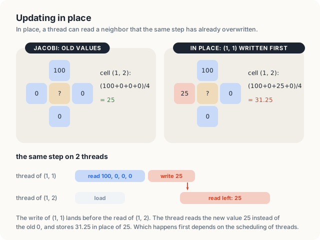
On a CPU, the update in place gives another well-defined method, called Gauss-Seidel iteration, which also converges. On a GPU, however, it gives no well-defined method at all, because the cells are updated by different threads. The thread of cell (1, 2) may read its left neighbor before or after the thread of cell (1, 1) writes it, and the order is decided by how the hardware schedules the 2 threads. The result can be 25, 31.25, or a mixture of both across the grid, and it can change from run to run. We run this variant in Section 19.5.
19.3.2 Which updates are independent
Recall the formula of Definition 19.3. Its right-hand side uses only values of step \(k\), and its left-hand side writes only values of step \(k + 1\). No update of a step therefore uses the result of another update of the same step. In step 2 of our plate, for example, cell (1, 2) needs the value of cell (1, 1) after step 1, which is 25, and not the value 31.25 that cell (1, 1) receives in step 2.
Key observation The 16 updates of a Jacobi step read only the grid of the previous step, so no update depends on another and all 16 can run at the same time, provided that no update overwrites a value of the previous step that another update still has to read.
The condition at the end of the observation is met by keeping the 2 grids of Jacobi apart. Every update reads from one grid and writes into the other, and the next step exchanges their roles. This arrangement has a name.
Definition 19.4 Ping-pong buffers. Ping-pong buffering keeps 2 buffers of the same size. Each step reads 1 buffer and writes the other, and after each step the 2 exchange roles, so that the buffer written last is the one read next.
Example. Step 1 of the plate reads buffer \(\mathsf{current}\) and writes buffer \(\mathsf{next}\); step 2 reads \(\mathsf{next}\) and writes \(\mathsf{current}\); step 3 reads \(\mathsf{current}\) again.
Exercises
19.7 Finish step 1 in place for row 1 and row 2 of the plate, visiting the cells row by row. Which
of the 16 values differ from Jacobi’s?
19.8 Suppose the cells of a step in place were visited column by column instead. Which value would
cell (1, 2) receive in step 1?
19.4 The parallel algorithm
19.4.1 Threads and blocks
A GPU runs 1 function many times at once. The terms below were introduced in Chapters 3 and 13. We restate them here because we use them throughout the rest of the chapter.
Definition 19.5 Kernel, thread, block, grid of blocks, warp. A kernel is a function that the GPU runs many times at once; each run is a thread, with its own position and its own variables. Threads are grouped into blocks of up to 1,024 threads that run on the same streaming multiprocessor (SM), share a fast on-chip memory and can wait for one another. The blocks of 1 launch form a grid of blocks. The SM issues instructions for 32 threads of a block at a time; such a group is a warp.
Example. For the plate, the program launches 1 block of 32 × 8 threads. Its 256 threads form 8 warps, 1 per row of the block.
The word “grid” now has 2 meanings, the grid of cells and the grid of blocks. In the rest of the chapter, we say “grid” for the cells and “the blocks of a launch” for the other meaning.
We give each cell its own thread. A thread finds its cell from 3 values that the GPU supplies: the position of its block among the blocks of the launch (\(\mathsf{blockIdx}\)), its position inside the block (\(\mathsf{threadIdx}\)), and the size of a block (\(\mathsf{blockDim}\)). We use blocks of 32 × 8 threads, so \(\mathsf{blockDim{.}x} = 32\) and \(\mathsf{blockDim{.}y} = 8\) that is, 32 threads along a row and 8 rows of threads. The thread at position (\(\mathsf{threadIdx{.}x}\), \(\mathsf{threadIdx{.}y}\)) of block (\(\mathsf{blockIdx{.}x}\), \(\mathsf{blockIdx{.}y}\)) then owns the cell
\[ \mathsf{row} = \mathsf{blockIdx{.}y} \cdot \mathsf{blockDim{.}y} + \mathsf{threadIdx{.}y}, \qquad \mathsf{col} = \mathsf{blockIdx{.}x} \cdot \mathsf{blockDim{.}x} + \mathsf{threadIdx{.}x}. \]
| Symbol | Meaning | Example: thread (4, 2) of block (1, 0) |
|---|---|---|
| \(\mathsf{blockDim{.}x}, \mathsf{blockDim{.}y}\) | width and height of a block in threads | 32, 8 |
| \(\mathsf{blockIdx{.}x}\), \(\mathsf{blockIdx{.}y}\) | column and row of the block among the blocks | 1, 0 |
| \(\mathsf{threadIdx{.}x}\), \(\mathsf{threadIdx{.}y}\) | column and row of the thread inside its block | 4, 2 |
| \(\mathsf{row}\) | row of the cell the thread owns | \(0 \cdot 8 + 2 = 2\) |
| \(\mathsf{col}\) | column of the cell the thread owns | \(1 \cdot 32 + 4 = 36\) |
The formula has a simple reading. Along a row, the blocks to the left of block \(\mathsf{blockIdx{.}x}\) cover \(\mathsf{blockIdx{.}x} \cdot \mathsf{blockDim{.}x}\) columns, and the thread lies \(\mathsf{threadIdx{.}x}\) columns further on. In the example of the table, block 1 has 1 block of 32 columns to its left, so its thread 4 owns column 36. The rows are counted in the same way.
A grid of \(W \times H\) cells needs \(\lceil W / \mathsf{blockDim{.}x} \rceil \times \lceil H / \mathsf{blockDim{.}y} \rceil\) blocks, where \(\lceil x \rceil\) denotes \(x\) rounded up to the next integer, so that a partly filled block at the edge is still counted. A grid of 4096 × 4096 cells needs \(4096 / 32 = 128\) blocks along a row and \(4096 / 8 = 512\) along a column. For the plate, \(\lceil 6 / 32 \rceil = \lceil 6 / 8 \rceil = 1\), so 1 block suffices. The threads of that block with \(\mathsf{col} \ge 6\) or \(\mathsf{row} \ge 6\) have no cell, and of the 36 threads that do have a cell, the 20 on the boundary have nothing to compute.
We choose blocks that are 32 threads wide because the 32 threads of a warp then lie along 1 row of the grid. When they read their neighbors, they read 32 neighboring values, 128 bytes, at the same time, and the hardware can serve such a read efficiently.
Definition 19.6 Coalesced access. Global memory moves data in sectors of 32 bytes (Chapter 7). A warp’s access is coalesced when its 32 threads read neighboring addresses, so that the 32 values arrive in as few sectors as possible.
Example. A warp reading 32 neighboring floats of a row, 128 bytes, needs 4 sectors when the row segment starts at a multiple of 32 bytes. A warp reading 32 floats of a column needs 32 sectors.
19.4.2 The kernel
Every thread executes the following procedure. The 2 grids \(u\) and \(v\) are 2 different buffers in global memory, the large memory of the GPU that every thread can read and write.
Jacobi-Kernel(\(u, v, W, H\))
- \(\mathsf{row} = \mathsf{blockIdx{.}y} \cdot \mathsf{blockDim{.}y} + \mathsf{threadIdx{.}y}\)
- \(\mathsf{col} = \mathsf{blockIdx{.}x} \cdot \mathsf{blockDim{.}x} + \mathsf{threadIdx{.}x}\)
- if \(\mathsf{row} \in [1, H - 1)\) and \(\mathsf{col} \in [1, W - 1)\) { // interior cells only
- \(v_{\mathsf{row},\mathsf{col}} = (u_{\mathsf{row}-1,\mathsf{col}} + u_{\mathsf{row}+1,\mathsf{col}} + u_{\mathsf{row},\mathsf{col}-1} + u_{\mathsf{row},\mathsf{col}+1}) / 4\)
- }
Jacobi-GPU(\(u, W, H, K\))
- copy \(u\) into 2 device buffers \(\mathsf{current}\) and \(\mathsf{next}\) // both hold the boundary
- for \(\mathsf{step} \in [0, K)\) {
- launch Jacobi-Kernel(\(\mathsf{current}, \mathsf{next}, W, H\)) on \(\lceil W/\mathsf{blockDim{.}x} \rceil \times \lceil H/\mathsf{blockDim{.}y} \rceil\) blocks
- exchange the names \(\mathsf{current}\) and \(\mathsf{next}\)
- }
- copy \(\mathsf{current}\) to the host
Jacobi-Kernel is the body of Jacobi-Step with its 2 loops removed. The position of the thread, computed in lines 1 and 2, plays the role of the loop variables \(\mathsf{row}\) and \(\mathsf{col}\). Line 3 lets only the threads of interior cells continue, and line 4 is line 3 of Jacobi-Step. Jacobi-GPU is Jacobi with the call of Jacobi-Step replaced by a launch of the kernel, and \(\mathsf{current}\) and \(\mathsf{next}\) are the 2 buffers on the device. Launches issued one after another on the same stream run in that order, so each launch starts only after every thread of the previous launch has written its value. The loop of the CPU is thus replaced by threads within a step, while the steps themselves still run one after another.
19.4.3 The work of 1 thread
Figure 19.5 follows the thread of cell (2, 2) through step 2. The thread reads 4 values from buffer \(\mathsf{current}\), which holds the grid after step 1, namely 25 above, 0 below, 0 to the left and 0 to the right. It then writes \(25 / 4 = 6.25\) into cell (2, 2) of buffer \(\mathsf{next}\). In total, the thread makes 4 reads from global memory and 1 write, and none of the values that it reads was written in the same step.
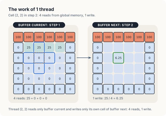
Over the whole step, the 16 interior threads of the plate read 64 values and write 16. A grid of 4096 × 4096 cells has 16.7 million interior threads per step, which read 67 million values, or 268 MB, and write 16.7 million values, or 67 MB. In Section 19.8, we will see that most of those reads never reach the memory chips.
Exercises
19.9 Which cell does thread (5, 3) of block (2, 1) own with blocks of 32 × 8 threads?
19.10 How many blocks of 32 × 8 threads cover a grid of 1000 × 1000 cells, and how many of their
threads have no cell?
19.11 Follow the thread of cell (1, 2) through step 2, as Figure 19.5 does for cell (2, 2).
19.5 Correctness
The kernel is correct only if the buffers are used as Jacobi-GPU prescribes. In this section, we break the prescription in two ways and run each broken variant. We then prove that the correct program computes Jacobi iteration exactly.
19.5.1 1 buffer for both arguments
Suppose that we launch the kernel with the same buffer as \(u\) and as \(v\). This is the
update in place of Section 19.3. In C++, the launch
jacobi<<<blocks, block>>>(current, current, width, height)
compiles without a warning. We ran it for 10 steps on the 4096 × 4096 plate, 3 times, and compared
each result with the result of 10 correct steps. The program printed the following counts.
in place, 4096 x 4096, run 1: 28420 of 16777216 cells differ from Jacobi after 10 steps
in place, 4096 x 4096, run 2: 28330 of 16777216 cells differ from Jacobi after 10 steps
in place, 4096 x 4096, run 3: 28464 of 16777216 cells differ from Jacobi after 10 steps
The number of wrong cells changes from run to run, as we predicted in Section 19.3. On the 6 × 6 plate, the same launch printed the correct values of Figure 19.3. There, all 36 cells belong to 1 block, and in our runs every thread of the block read its neighbors before any of them wrote. Nothing in the hardware guarantees that order, however. A test on a small grid therefore cannot show the error. The error appears where 1 block reads cells that another block, running earlier or later, writes.
In Rust, the same mistake does not compile. The kernel takes the old grid as &[f32] and the new
one as a DisjointSlice, which the launch builds from a &mut borrow of a buffer. Passing the
same buffer as both arguments borrows it as shared and as mutable at the same time, which the
borrow checker rejects with the following message.
error[E0502]: cannot borrow `current` as mutable because it is also borrowed as immutable
--> src/main.rs:154:64
|
154 | module.jacobi(&stream, &small, ¤t, RowWidth::new(&mut current, width as u32))?;
| ------ -------- ^^^^^^^^^^^^ mutable borrow occurs here
| | |
| | immutable borrow occurs here
| immutable borrow later used by call
19.5.2 A buffer without the boundary
The compiler can check that the 2 arguments are different buffers, but it cannot check what a buffer holds. Suppose that line 1 of Jacobi-GPU copies the plate into \(\mathsf{current}\) only, and that \(\mathsf{next}\) is created filled with 0. The kernel never writes a boundary cell, so the top row of \(\mathsf{next}\) stays at 0. Step 1 is unaffected, because it reads \(\mathsf{current}\). Step 2, however, reads \(\mathsf{next}\), whose top edge is cold, and cell (1, 1) becomes \((0 + 0 + 0 + 25) / 4 = 6.25\) instead of 31.25, as shown in Figure 19.6. We ran this variant, and it printed the following grids.
  zeroed second buffer, after step 2
     100.00  100.00  100.00  100.00  100.00  100.00
       0.00    6.25   12.50   12.50    6.25    0.00
       0.00    6.25    6.25    6.25    6.25    0.00
       0.00    0.00    0.00    0.00    0.00    0.00
       0.00    0.00    0.00    0.00    0.00    0.00
       0.00    0.00    0.00    0.00    0.00    0.00
  zeroed second buffer, after step 200
     100.00  100.00  100.00  100.00  100.00  100.00
       0.00   11.55   21.76   21.76   11.55    0.00
       0.00   13.88   17.55   17.55   13.88    0.00
       0.00    4.79    8.45    8.45    4.79    0.00
       0.00    2.45    3.58    3.58    2.45    0.00
       0.00    0.00    0.00    0.00    0.00    0.00
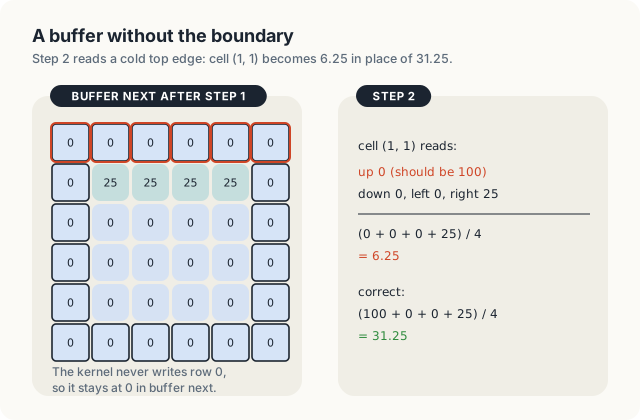
The grid printed after step 2 shows 100 in its top row. The program printed buffer \(\mathsf{current}\), which holds the boundary, while the step itself had read the cold top row of \(\mathsf{next}\). The iteration still converges, but to the answer of a different problem, in which the top edge is hot only in every second step. After 200 steps, cell (2, 2) holds 17.55, whereas the correct value is 32.95. No error is reported, and only a comparison with known values exposes the mistake.
19.5.3 A proof of correctness
We can now prove that the correct program computes Jacobi iteration. The proof follows the 2 buffers at the start of each pass through the loop of Jacobi-GPU, as shown in Figure 19.7.
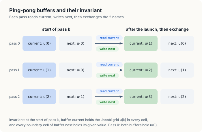
Theorem 19.1 When Jacobi-GPU finishes, buffer \(\mathsf{current}\) holds the grid \(u^{(K)}\) of Definition 19.3, in every cell.
Proof. We show that the loop of lines 2 to 5 maintains the following invariant: at the start of pass \(k\), (i) buffer \(\mathsf{current}\) holds \(u^{(k)}\) in every cell, and (ii) every boundary cell of \(\mathsf{next}\) holds its given value.
Initialization. Before pass 0, line 1 has copied the starting grid \(u = u^{(0)}\) into both buffers. Both parts of the invariant therefore hold.
Maintenance. Assume that the invariant holds at the start of pass \(k\). The launch in line 3 reads only \(\mathsf{current}\) and writes only interior cells of \(\mathsf{next}\), and \(\mathsf{current}\) and \(\mathsf{next}\) are different buffers, so no thread reads a value that another thread of the launch writes. Every thread therefore reads values of \(u^{(k)}\), and line 4 of Jacobi-Kernel stores \(u^{(k+1)}_{r,c}\) into each interior cell of \(\mathsf{next}\). The boundary cells of \(\mathsf{next}\) are not written, so they still hold the given values, which are also the boundary values of \(u^{(k+1)}\). Hence, \(\mathsf{next}\) holds \(u^{(k+1)}\) in every cell. Buffer \(\mathsf{current}\) was not written, so its boundary cells still hold the given values. Line 4 exchanges the names, after which (i) and (ii) hold for pass \(k + 1\). The next launch starts only after this one has finished, because launches on 1 stream run in order.
Termination. The loop ends after \(K\) passes, so \(\mathsf{current}\) holds \(u^{(K)}\), and line 6 copies it to the host.
Each broken variant of this section violates 1 step of the proof. The launch with 1 buffer violates the condition that \(\mathsf{current}\) and \(\mathsf{next}\) are different buffers in the maintenance step. The zeroed buffer violates part (ii) of the invariant at initialization, and the proof then fails at the first exchange, when \(\mathsf{next}\) becomes the buffer that the next step reads.
Rule A Jacobi step reads 1 buffer and writes the other, never the same one, and both buffers hold the boundary values before the first step.
Exercises
19.12 In the zeroed-buffer variant, compute cell (1, 2) after step 2 by hand and compare it with
the output above.
19.13 Suppose the kernel also wrote the boundary cells, copying them from \(u\) to \(v\). Would
the zeroed second buffer still give a wrong answer? Which part of the invariant would the proof no
longer need?
19.14 The output above shows the in-place launch with 3 different results. Why can a block of the
4096 × 4096 grid read a value that another block has already overwritten, while the single block of
the 6 × 6 plate did not?
19.6 Implementation
19.6.1 The kernel
Listing 19.1 shows the kernel in both languages. We let each thread compute its position, which is lines 1
and 2 of Jacobi-Kernel, keep only interior cells, which is line 3, and store the mean of its 4
neighbors, which is line 4. In the flat array, the cell itself is element
center = row * width + col.
Its neighbors above and below are \(W\) elements away, at center - width and center + width, and
those to the left and right are at center - 1 and center + 1. For cell (2, 2) of the plate,
center is
\(2 \cdot 6 + 2 = 14\), and the 4 neighbors are elements 8, 20, 13 and 15. Both versions add the
4 values in the same order and multiply by 0.25 last, as the CPU reference of the programs does,
so that the GPU and the CPU round identically.
Listing 19.1 One Jacobi step, one thread per cell.
mod kernels {
    // ...
    /// 1 Jacobi step: each interior cell of `new` gets the mean of 4 neighbors in `old`.
    #[kernel]
    #[launch_contract(domain = 2, block = (32, 8, 1))]
    pub fn jacobi(old: &[f32], mut new: DisjointSlice<f32, Runtime2DIndex>) {
        let width = new.row_width() as usize;
        let height = new.len() / width;

        if let Some(idx) = thread::index_2d_runtime(&new) {
            let (row, col) = (idx.row(), idx.col());
            let interior = row >= 1 && row + 1 < height && col >= 1 && col + 1 < width;

            if interior {
                let center = row * width + col;
                let (above, below) = (old[center - width], old[center + width]);
                let (left, right) = (old[center - 1], old[center + 1]);
                let sum = above + below + left + right;

                if let Some(cell) = new.get_mut(idx) {
                    *cell = 0.25 * sum;
                }
            }
        }
    }
    // ...
}
// 1 Jacobi step: each interior cell of `next` gets the mean of its 4 neighbors in `old`.
__global__ void jacobi(const float* __restrict__ old, float* __restrict__ next,
int width, int height)
{
int row = blockIdx.y * blockDim.y + threadIdx.y;
int col = blockIdx.x * blockDim.x + threadIdx.x;
bool interior = row >= 1 && row + 1 < height && col >= 1 && col + 1 < width;
if (interior) {
int center = row * width + col;
float above = old[center - width];
float below = old[center + width];
float sum = above + below + old[center - 1] + old[center + 1];
next[center] = 0.25f * sum;
}
}
The two versions differ in how they state that the 2 grids do not overlap. The C++ kernel receives 2
raw pointers and marks them __restrict__, which is a promise to the compiler that no element is
reached through both pointers. The compiler does not check this promise. The Rust kernel receives
the old grid as a shared slice, &[f32], and the new grid as a
DisjointSlice<f32, Runtime2DIndex>, a slice that each thread may write only at its own position.
The Rust kernel obtains that position in 3 steps. First, the host attaches the row width to the
buffer with RowWidth::new, and on the device, row_width() returns it. Second,
thread::index_2d_runtime(&new) returns the thread’s (row, column) position as an index that only
this thread holds. Third, get_mut turns that index into element row * width + col, checks it
against the length of the slice, and returns a mutable reference to the element. Since no 2
threads hold the same index, no 2 threads can write the same element, and the write needs no
unsafe block. This is the same guarantee that the borrow checker enforced on the host in
Section 19.5.1, where it rejected 1 buffer passed as both arguments.
19.6.2 The host loop
Listing 19.2 implements Jacobi-GPU for the plate, that is, lines 1 to 5 of the pseudocode. It fills both buffers from the same host grid, launches 100 steps, exchanges the 2 buffers after each step, and prints the grid after steps 1, 2 and 100.
Listing 19.2 100 steps on the 6 × 6 plate, with the 2 buffers exchanged after each step.
fn main() -> Result<(), Error> {
// ...
// 1. The 6 x 6 plate of the text, small enough to check by hand.
let (width, height) = (6, 6);
let start = initial_grid(width, height);
let mut current = DeviceBuffer::from_host(&stream, &start)?;
let mut next = DeviceBuffer::from_host(&stream, &start)?;
let small = module.prepare_jacobi(grid_2d(width, height))?;
println!("1. 6 x 6 plate, top edge at {HOT}");
let mut changes = Vec::new();
for step in 1..=100 {
module.jacobi(&stream, &small, ¤t, RowWidth::new(&mut next, width as u32))?;
std::mem::swap(&mut current, &mut next);
let (new, old) = (current.to_host_vec(&stream)?, next.to_host_vec(&stream)?);
changes.push(rms_change(&new, &old));
if step <= 2 || step == 100 {
print_grid(&format!("after step {step}"), &new, width);
}
}
// ...
}int main()
{
// ...
// 1. The 6 x 6 plate of the text, small enough to check by hand.
int width = 6;
int height = 6;
Grid start = initialGrid(width, height);
float* current;
float* next;
std::tie(current, next) = deviceGrids(start);
std::printf("1. 6 x 6 plate, top edge at %.0f\n", HOT);
std::vector<double> changes;
for (int step = 1; step <= 100; ++step) {
jacobi<<<blocksFor(width, height), block>>>(current, next, width, height);
std::swap(current, next);
Grid newer = toHost(current, width, height);
Grid older = toHost(next, width, height);
changes.push_back(rmsChange(newer, older));
if (step <= 2 || step == 100) {
char label[32];
std::snprintf(label, sizeof label, "after step %d", step);
printGrid(label, newer, width);
}
}
// ...
}
Both buffers are filled from the same host grid start, which is line 1 of Jacobi-GPU and
establishes part (ii) of the invariant. The exchange of line 4 moves no grid data. In C++,
std::swap(current, next) exchanges 2 pointers of 8 bytes each. In Rust, std::mem::swap(&mut current, &mut next)
exchanges 2 DeviceBuffer values, which are small handles of 40 bytes that hold the device address,
the length and a reference to the context, while the grids themselves stay where they are in
device memory. For comparison, a step on a 4096 × 4096 grid moves at least 134 MB, whereas the
exchange moves 80 bytes of host memory.
19.6.3 Running the example
Both programs print the same values. The Rust program prints the following output.
$ cargo oxide run
GPU: Orin, 8 SMs
1. 6 x 6 plate, top edge at 100
after step 1
100.00 100.00 100.00 100.00 100.00 100.00
0.00 25.00 25.00 25.00 25.00 0.00
0.00 0.00 0.00 0.00 0.00 0.00
0.00 0.00 0.00 0.00 0.00 0.00
0.00 0.00 0.00 0.00 0.00 0.00
0.00 0.00 0.00 0.00 0.00 0.00
after step 2
100.00 100.00 100.00 100.00 100.00 100.00
0.00 31.25 37.50 37.50 31.25 0.00
0.00 6.25 6.25 6.25 6.25 0.00
0.00 0.00 0.00 0.00 0.00 0.00
0.00 0.00 0.00 0.00 0.00 0.00
0.00 0.00 0.00 0.00 0.00 0.00
after step 100
100.00 100.00 100.00 100.00 100.00 100.00
0.00 45.45 59.47 59.47 45.45 0.00
0.00 22.35 32.95 32.95 22.35 0.00
0.00 10.98 17.05 17.05 10.98 0.00
0.00 4.55 7.20 7.20 4.55 0.00
0.00 0.00 0.00 0.00 0.00 0.00
Every value of steps 1 and 2 agrees with the values that we computed by hand in Section 19.2.1.
The program also runs the same 100 steps on the CPU with the function cpu_step, and it reports
same bits as the CPU after 100 steps: true. The 2 computations therefore agree in every bit of
every cell. This is possible because each cell is computed by the same 3 additions in the same
order, followed by the same multiplication, and IEEE 754 single-precision arithmetic rounds such a
sequence identically on both processors.
Exercises
19.15 Change the programs to print the grid after step 3 and compare it with your answer to
Exercise 19.4.
19.16 The Rust launch passes ¤t and RowWidth::new(&mut next, ...). Explain why the borrow checker
accepts this call but rejects the one of Section 19.5.1.
19.7 Convergence
19.7.1 Measuring the change
After 100 steps, the plate agrees with the final temperatures to 2 decimal places. In general, however, the final temperatures are not known in advance, so a solver must decide by itself when to stop. It does so by measuring how much a step still changes the grid. When a step hardly changes any value, the grid is close to the state in which every cell equals the mean of its neighbors.
Definition 19.7 RMS change. The root-mean-square (RMS) change of a step from grid \(u\) to grid \(v\) of \(N\) cells is
\[ \Delta = \sqrt{\frac{1}{N} \sum_{i \in [0, N)} (v_i - u_i)^2 }. \]
Example. Step 1 of the plate changes 4 of the 36 cells by 25 each: \(\Delta = \sqrt{4 \cdot 625 / 36} = 8.33\) degrees.
| Symbol | Meaning | Step 1 of the plate |
|---|---|---|
| \(N\) | number of cells of the grid | 36 |
| \(i\) | position of a cell in the flat array | 0 to 35 |
| \(u_i\), \(v_i\) | value of cell \(i\) before and after the step | 0 and 25 for the 4 cells of row 1 |
| \((v_i - u_i)^2\) | square of the change of cell \(i\) | 625 for those 4 cells, 0 for the rest |
| \(\Delta\) | square root of the mean of the squares: a typical change per cell | 8.33 |
The squares make every change count as positive, so that a rise in 1 cell cannot cancel a fall in another, and the square root at the end returns the result to degrees.
Both programs copy the 2 buffers to the host after every step of the plate and compute the RMS change there. A 6 × 6 grid occupies only 144 bytes, so the copy costs microseconds. The programs print the change and its ratio to the change of the step before, as follows.
RMS change per step, and its ratio to the step before
step 1 8.33e+00
step 2 3.90e+00 ratio 0.4677
step 3 2.52e+00 ratio 0.6478
step 4 1.82e+00 ratio 0.7192
step 10 4.48e-01 ratio 0.8075
step 20 5.38e-02 ratio 0.8090
step 40 7.75e-04 ratio 0.8086
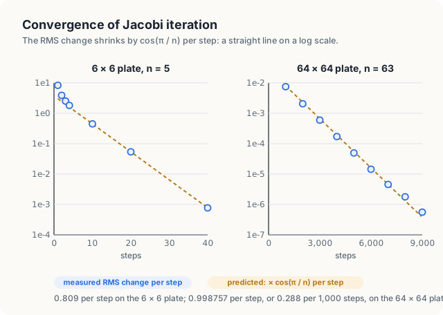
After the first few steps, the change shrinks by the same factor in every step, 0.809.
19.7.2 The rate of convergence
This factor can be predicted. Let the error of a grid be its difference from the final temperatures, cell by cell. A Jacobi step leaves the final temperatures unchanged, since each of them already equals the mean of its neighbors. A step therefore applies the same averaging to the error that it applies to the grid, and the error after a step is the mean of the neighboring errors before it. An error pattern that varies quickly from cell to cell, for example \(+1\) and \(-1\) in alternating cells, is averaged away in a few steps, because neighboring values cancel. The pattern that survives longest is the smoothest one that is 0 on the boundary, a single bump that is largest in the middle of the plate. On a grid whose cells are numbered 0 to \(n\) along each side, this pattern is
\[ e_{r,c} = \sin\frac{\pi r}{n} \, \sin\frac{\pi c}{n}. \]
| Symbol | Meaning | On the 6 × 6 plate |
|---|---|---|
| \(n\) | number of the last row and column; the boundary lies at 0 and \(n\) | 5 |
| \(e_{r,c}\) | error of cell \((r, c)\) in the slowest pattern | 0 on the boundary, largest in the center |
| \(\sin(\pi r / n)\) | a half wave along the rows, 0 at \(r = 0\) and at \(r = n\) | \(\sin(\pi/5) = 0.588\) at \(r = 1\) |
Let us apply 1 step to this pattern. The 2 neighbors of cell \((r, c)\) in its column hold \(\sin(\pi(r - 1)/n)\) and \(\sin(\pi(r + 1)/n)\), each multiplied by the same column factor \(\sin(\pi c / n)\). By the identity \(\sin(x - y) + \sin(x + y) = 2 \sin x \cos y\), their sum is \(2\cos(\pi/n)\) times the value of the cell, and the same holds for the 2 neighbors in its row. The sum of the 4 neighbors is therefore \(4\cos(\pi/n)\) times the value of the cell, their mean is \(\cos(\pi/n)\) times that value, and 1 step multiplies the whole pattern by
\[ \rho = \cos\frac{\pi}{n}. \]
Our plate has \(n = 5\), and \(\cos(\pi/5) = 0.8090\), which is the ratio that the programs measured from step 10 on. The early ratios are smaller, because the rougher error patterns, which shrink faster, have not yet died out.
The same programs then iterate a 64 × 64 plate, for which \(n = 63\), until the RMS change of a step falls below \(10^{-6}\) degrees. They measure the change every 1,000 steps and print the following values.
2. 64 x 64 plate until the RMS change per step is below 1e-6
step 1000 RMS change 7.49e-03
step 2000 RMS change 2.06e-03
step 3000 RMS change 5.95e-04
step 4000 RMS change 1.71e-04
step 5000 RMS change 4.95e-05
step 6000 RMS change 1.44e-05
step 7000 RMS change 4.57e-06
step 8000 RMS change 1.79e-06
step 9000 RMS change 5.59e-07
largest difference from the CPU after 9000 steps: 0.00e+00
The prediction is \(\rho = \cos(\pi/63) = 0.998757\) per step, so 1,000 steps multiply the change by \(0.998757^{1000} = 0.288\). The measured ratios between consecutive lines are \(2.06 / 7.49 = 0.275\), \(0.595 / 2.06 = 0.289\), \(0.171 / 0.595 = 0.287\) and \(0.0495 / 0.171 = 0.289\), in close agreement with the prediction, as Figure 19.8 shows. After step 7,000, the ratio drifts upward, to 0.39 and 0.31, because the changes have become smaller than the rounding error of single-precision values near 50, which is about \(4 \times 10^{-6}\) degrees.
The prediction also gives the cost of the method on a large grid. When \(\rho\) is close to 1, each step removes only the small fraction \(1 - \rho\) of the remaining error, so reducing the error by a factor of \(e = 2.718\) takes about \(1 / (1 - \rho)\) steps. For large \(n\), \(1 - \cos(\pi/n)\) is close to \(\pi^2 / (2n^2)\), so this number of steps is about \(2n^2/\pi^2\). It is 5 for our plate, about 800 for \(n = 63\), and about 3.4 million for a grid of 4096 × 4096 cells. The number of steps grows with the square of the width, so large solvers use Jacobi steps as one part of faster methods, such as multigrid, which apply a few Jacobi steps on a series of coarser grids. A fast Jacobi step is the building block of those methods, and in the rest of this chapter and in the next, we measure how fast a step can be.
Exercises
19.17 Predict \(\rho\) and the factor per 1,000 steps for a 128 × 128 plate. Change the programs
and compare.
19.18 About how many steps reduce the error of the 64 × 64 plate by a factor of 1,000?
19.8 Memory traffic and measurements
19.8.1 Arithmetic intensity
Each update performs 4 floating-point operations (FLOP). To judge whether this is much or little, we compare it with the number of bytes that the update must move. Every old value must be read at least once, and every new value must be written once. The least that any step can move is therefore 1 read and 1 write of 4 bytes per cell, 8 bytes in total.
Definition 19.8 Arithmetic intensity, memory-bound. The arithmetic intensity of a computation is the number of floating-point operations it performs per byte it moves to or from memory. A kernel is memory-bound on a GPU when its arithmetic intensity lies below the GPU’s ridge point, its peak arithmetic rate divided by its memory bandwidth (Chapter 2); its speed is then set by the bytes it moves, not by the operations it performs.
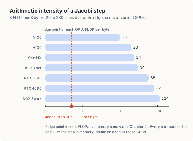
Example. A Jacobi step performs 4 FLOP per cell and moves at least 8 bytes per cell, so its arithmetic intensity is at most \(4 / 8 = 0.5\) FLOP per byte.
The ridge point is the arithmetic intensity at which a kernel would keep both the arithmetic units and the memory fully busy. The ridge points of the GPUs compared in Chapter 2 range from about 10 FLOP per byte for the A100 to about 114 FLOP per byte for the DGX Spark. The Jetson Orin NX lies at about 24, and the Jetson AGX Thor at about 30, as Figure 19.9 shows. A Jacobi step lies below every one of them by a factor of 20 or more, so it is memory-bound on every GPU of the table. Its speed is therefore best measured by its effective bandwidth, the 8 bytes per cell that a step must move divided by the time of the step. Since a copy of the grid moves the same 8 bytes per cell, a step can be no faster than a copy.
19.8.2 Measurements
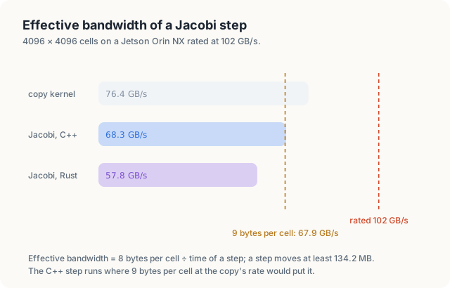
The measurements come from a Jetson Orin NX, an integrated GPU with 8 SMs and 102 GB/s of memory bandwidth. Both programs time a step on a 4096 × 4096 grid, which occupies 64 MiB per buffer. This is far larger than the 2 MiB L2 cache of the measured GPU, so the grid must come from memory. Each program first runs the kernel for 0.4 s, because these GPUs raise their clock frequency only under sustained load, and then averages 50 calls. Repeated runs differ by 10 to 20%. On the measured GPU, the C++ program printed
3. 4096 x 4096 plate, 8 bytes per cell per step (1 read, 1 write)
copy kernel 1.756 ms 76.4 GB/s
jacobi 1.966 ms 68.3 GB/s
PASSED
and the Rust program printed
3. 4096 x 4096 plate, 8 bytes per cell per step (1 read, 1 write)
copy kernel 1.784 ms 75.2 GB/s
jacobi 2.322 ms 57.8 GB/s
PASSED
The following table and Figure 19.10 collect these numbers. The last column gives the effective bandwidth of each kernel as a share of the bandwidth of the copy.
| Kernel | Time per step | Effective bandwidth | Share of the copy |
|---|---|---|---|
| copy, C++ | 1.756 ms | 76.4 GB/s | 100% |
| Jacobi step, C++ | 1.966 ms | 68.3 GB/s | 89% |
| Jacobi step, Rust | 2.322 ms | 57.8 GB/s | 76% |
19.8.3 Why the step runs at 89% of a copy
The copy reaches 76.4 GB/s, which is 75% of the rated 102 GB/s. In Chapter 7, we saw that no kernel reaches the rated figure, so the copy, not the rating, is the ceiling for a step. The C++ step reaches 89% of the copy. This is more than we should expect at first sight. If every one of its 4 reads per cell went to memory, a step would move 16 bytes of reads and 4 bytes of writes, 20 bytes per cell, and it would take at least \(20 / 8 = 2.5\) times as long as the copy, that is, 4.4 ms. It took 1.97 ms.
Let us compute what that time would require. Requesting 20 bytes for each of the 16.7 million cells in 1.966 ms is a rate of \(20 \cdot 16.7 \times 10^6 / 1.966 \times 10^{-3}\) = 171 GB/s, which is 1.7 times the 102 GB/s that the memory can deliver at all. At most 102 of every 171 requested bytes can therefore have come from memory, and at least \(1 - 102/171 = 40\%\) of them must have come from the L1 and L2 caches, the on-chip memories that keep recently read values.
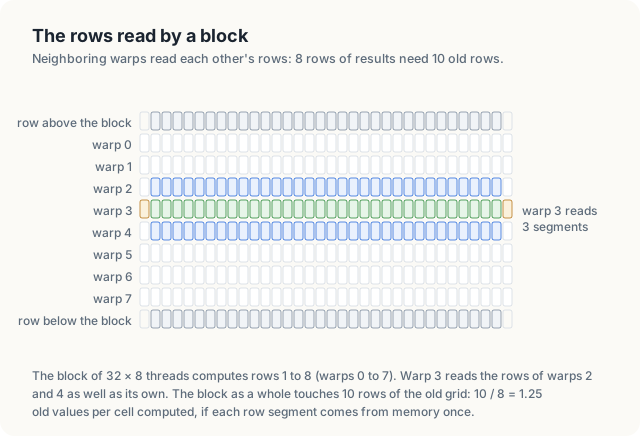
The caches find those values because neighboring threads read neighboring rows, as Figure 19.11 shows. The 32 threads of a warp read 3 row segments of the old grid: the row above, their own row with 1 extra cell at each end, and the row below. The 8 warps of a block cover 8 consecutive rows, so the row above warp 1 is the row of warp 0, and the row below warp 1 is the row of warp 2. A block of 32 × 8 threads therefore needs only 10 different row segments of the old grid, its own 8 rows and 1 more on each side. If each segment is read from memory once, a block reads \(10 / 8 = 1.25\) old values per cell and writes 1, which is 9 bytes per cell instead of 8. At the copy’s rate, 9 bytes per cell take \(1.756 \cdot 9 / 8 = 1.98\) ms, which agrees with the measured 1.966 ms.
The step is thus close to the best it can be. It moves about 9 bytes per cell where 8 are needed, and its speed follows from that count. In Chapter 20, we ask whether a block can do better by copying its 10 rows into shared memory itself.
19.8.4 Why the Rust step is slower
The Rust kernel runs at 57.8 GB/s, 85% of the speed of the C++ kernel, although it reads and writes
the same cells. Its memory traffic is the same, but its integer work is not. The C++ kernel computes
positions in 32-bit int. The Rust kernel computes them in 64-bit usize, derives the height with
a 64-bit division, new.len() / width, and checks each index against the length of its slice. To
separate these costs, we changed only the C++ kernel, so that it used 64-bit positions and the same
division of the length by the width. It then ran at 58.9 GB/s, the speed of the Rust kernel. A
memory-bound kernel is therefore not free of arithmetic. With only 4 floating-point operations per
cell, the integer instructions that compute positions and check bounds make up most of the kernel,
and a 64-bit division, which the GPU performs as a sequence of many instructions, delays the loads.
Exercises
19.19 Rewrite the Rust kernel so that it computes positions in u32 and receives the height as an
argument, then measure it. How close does it come to the C++ kernel?
19.20 Change the block shape of both programs to 16 × 16 and predict, with the row count of
Section 19.8.3, how many old values a block reads per cell. Then measure.
19.9 The complete programs
Listing 19.3 The complete Rust program. code/oxide/ch19_stencil/src/main.rs
//! Chapter 19: Jacobi iteration for the Laplace equation, 1 thread per cell.
//!
//! cargo oxide run
use std::sync::Arc;
use std::time::Instant;
use cuda_core::{CudaContext, CudaStream, DeviceBuffer, LaunchConfig1D, LaunchConfig2D};
use cuda_device::thread::Runtime2DIndex;
use cuda_device::{DisjointSlice, cuda_module, kernel, launch_contract, thread};
use cuda_host::RowWidth;
const BLOCK_WIDTH: usize = 32; // 1 warp along a row of the grid
const BLOCK_HEIGHT: usize = 8; // 8 warps, 256 threads
const HOT: f32 = 100.0; // the top edge; the other edges are held at 0
type Error = Box<dyn std::error::Error>;
#[cuda_module]
mod kernels {
use super::*;
/// 1 Jacobi step: each interior cell of `new` gets the mean of 4 neighbors in `old`.
#[kernel]
#[launch_contract(domain = 2, block = (32, 8, 1))]
pub fn jacobi(old: &[f32], mut new: DisjointSlice<f32, Runtime2DIndex>) {
let width = new.row_width() as usize;
let height = new.len() / width;
if let Some(idx) = thread::index_2d_runtime(&new) {
let (row, col) = (idx.row(), idx.col());
let interior = row >= 1 && row + 1 < height && col >= 1 && col + 1 < width;
if interior {
let center = row * width + col;
let (above, below) = (old[center - width], old[center + width]);
let (left, right) = (old[center - 1], old[center + 1]);
let sum = above + below + left + right;
if let Some(cell) = new.get_mut(idx) {
*cell = 0.25 * sum;
}
}
}
}
/// A copy: 1 read and 1 write per cell, the least traffic a step can have.
#[kernel]
#[launch_contract(domain = 1, block = (256, 1, 1))]
pub fn copy(input: &[f32], mut out: DisjointSlice<f32>) {
let idx = thread::index_1d();
let index = idx.get();
if let Some(out_cell) = out.get_mut(idx) {
*out_cell = input[index];
}
}
}
/// A plate of `width` x `height` cells: the top row at HOT, every other cell at 0.
fn initial_grid(width: usize, height: usize) -> Vec<f32> {
let mut grid = vec![0.0; width * height];
grid[..width].fill(HOT);
grid
}
/// 1 Jacobi step on the CPU, the reference for the GPU kernel.
fn cpu_step(old: &[f32], new: &mut [f32], width: usize) {
let height = old.len() / width;
for row in 1..height - 1 {
for col in 1..width - 1 {
let center = row * width + col;
let (above, below) = (old[center - width], old[center + width]);
let (left, right) = (old[center - 1], old[center + 1]);
let sum = above + below + left + right;
new[center] = 0.25 * sum;
}
}
}
/// The root-mean-square difference between 2 grids, over all cells.
fn rms_change(new: &[f32], old: &[f32]) -> f64 {
let squares: f64 = new
.iter()
.zip(old)
.map(|(new_value, old_value)| f64::from(new_value - old_value).powi(2))
.sum();
(squares / new.len() as f64).sqrt()
}
/// A number in the style of C's %.2e, so that both programs print the same text.
fn sci(v: f64) -> String {
let exponent = if v == 0.0 { 0 } else { v.abs().log10().floor() as i32 };
format!("{:.2}e{exponent:+03}", v / 10f64.powi(exponent))
}
fn print_grid(label: &str, grid: &[f32], width: usize) {
println!(" {label}");
for row in grid.chunks(width) {
let cells: Vec<String> = row.iter().map(|v| format!("{v:7.2}")).collect();
println!(" {}", cells.join(" "));
}
}
/// Enough 32 x 8 blocks to cover a grid of `width` x `height` cells, 1 thread per cell.
fn grid_2d(width: usize, height: usize) -> LaunchConfig2D {
let blocks_x = width.div_ceil(BLOCK_WIDTH) as u32;
let blocks_y = height.div_ceil(BLOCK_HEIGHT) as u32;
LaunchConfig2D::new((blocks_x, blocks_y), (BLOCK_WIDTH as u32, BLOCK_HEIGHT as u32), 0)
}
/// Average time of `runs` calls of `launch`, in milliseconds, after 0.4 s of warm-up.
fn time_ms(
stream: &Arc<CudaStream>,
runs: u32,
mut launch: impl FnMut() -> Result<(), Error>,
) -> Result<f64, Error> {
let warm = Instant::now();
while warm.elapsed().as_secs_f64() < 0.4 {
launch()?;
stream.synchronize()?;
}
let start = Instant::now();
for _ in 0..runs {
launch()?;
}
stream.synchronize()?;
Ok(start.elapsed().as_secs_f64() * 1e3 / runs as f64)
}
fn main() -> Result<(), Error> {
let ctx = CudaContext::new(0)?;
let stream = ctx.default_stream();
// SAFETY: the loaded code was compiled from the `kernels` module above.
let module = unsafe { kernels::load(&ctx)? };
let name = ctx.device_name()?;
let sms = ctx.multiprocessor_count()?;
println!("GPU: {name}, {sms} SMs");
// 1. The 6 x 6 plate of the text, small enough to check by hand.
let (width, height) = (6, 6);
let start = initial_grid(width, height);
let mut current = DeviceBuffer::from_host(&stream, &start)?;
let mut next = DeviceBuffer::from_host(&stream, &start)?;
let small = module.prepare_jacobi(grid_2d(width, height))?;
println!("1. 6 x 6 plate, top edge at {HOT}");
let mut changes = Vec::new();
for step in 1..=100 {
module.jacobi(&stream, &small, ¤t, RowWidth::new(&mut next, width as u32))?;
std::mem::swap(&mut current, &mut next);
let (new, old) = (current.to_host_vec(&stream)?, next.to_host_vec(&stream)?);
changes.push(rms_change(&new, &old));
if step <= 2 || step == 100 {
print_grid(&format!("after step {step}"), &new, width);
}
}
println!(" RMS change per step, and its ratio to the step before");
println!(" step {:3} {:>9}", 1, sci(changes[0]));
for step in [2, 3, 4, 10, 20, 40] {
let ratio = changes[step - 1] / changes[step - 2];
println!(" step {step:3} {:>9} ratio {ratio:.4}", sci(changes[step - 1]));
}
let mut cpu_a = start.clone();
let mut cpu_b = start.clone();
for _ in 0..100 {
cpu_step(&cpu_a, &mut cpu_b, width);
std::mem::swap(&mut cpu_a, &mut cpu_b);
}
let small_same = current.to_host_vec(&stream)? == cpu_a;
println!(" same bits as the CPU after 100 steps: {small_same}");
// 2. A 64 x 64 plate, iterated until the RMS change per step is below 1e-6.
let (width, height) = (64, 64);
let start = initial_grid(width, height);
let mut current = DeviceBuffer::from_host(&stream, &start)?;
let mut next = DeviceBuffer::from_host(&stream, &start)?;
let step = module.prepare_jacobi(grid_2d(width, height))?;
println!("2. 64 x 64 plate until the RMS change per step is below 1e-6");
let mut steps = 0;
loop {
module.jacobi(&stream, &step, ¤t, RowWidth::new(&mut next, width as u32))?;
std::mem::swap(&mut current, &mut next);
steps += 1;
if steps % 1000 == 0 {
let (new, old) = (current.to_host_vec(&stream)?, next.to_host_vec(&stream)?);
let rms = rms_change(&new, &old);
println!(" step {steps:5} RMS change {}", sci(rms));
if rms < 1e-6 {
break;
}
}
}
let field = current.to_host_vec(&stream)?;
let mut cpu_a = start.clone();
let mut cpu_b = start.clone();
for _ in 0..steps {
cpu_step(&cpu_a, &mut cpu_b, width);
std::mem::swap(&mut cpu_a, &mut cpu_b);
}
let differences = field.iter().zip(&cpu_a).map(|(gpu, cpu)| (gpu - cpu).abs());
let diff = differences.fold(0.0, f32::max);
let shown = sci(f64::from(diff));
println!(" largest difference from the CPU after {steps} steps: {shown}");
// 3. A 4096 x 4096 plate: time per step and effective bandwidth.
let (width, height) = (4096, 4096);
let cells = width * height;
let start = initial_grid(width, height);
let mut current = DeviceBuffer::from_host(&stream, &start)?;
let mut next = DeviceBuffer::from_host(&stream, &start)?;
let big = module.prepare_jacobi(grid_2d(width, height))?;
let copy = module.prepare_copy(LaunchConfig1D::new((cells / 256) as u32, 256, 0))?;
let copy_once = || Ok(module.copy(&stream, ©, ¤t, &mut next)?);
let ms_copy = time_ms(&stream, 50, copy_once)?;
let ms_jacobi = time_ms(&stream, 50, || {
module.jacobi(&stream, &big, ¤t, RowWidth::new(&mut next, width as u32))?;
module.jacobi(&stream, &big, &next, RowWidth::new(&mut current, width as u32))?;
Ok(())
})? / 2.0;
let gb = |ms: f64| (2 * cells * 4) as f64 / 1e9 / (ms / 1e3);
println!("3. 4096 x 4096 plate, 8 bytes per cell per step (1 read, 1 write)");
println!(" copy kernel {ms_copy:6.3} ms {:6.1} GB/s", gb(ms_copy));
println!(" jacobi {ms_jacobi:6.3} ms {:6.1} GB/s", gb(ms_jacobi));
let passed = small_same && diff == 0.0;
println!("{}", if passed { "PASSED" } else { "FAILED" });
Ok(())
}// Chapter 19: Jacobi iteration for the Laplace equation, 1 thread per cell.
// Build: nvcc -O3 -arch=native stencil.cu -o stencil
#include <chrono>
#include <cmath>
#include <cstdio>
#include <cstdlib>
#include <tuple>
#include <utility>
#include <vector>
#include <cuda_runtime.h>
using Grid = std::vector<float>;
const int BLOCK_WIDTH = 32; // 1 warp along a row of the grid
const int BLOCK_HEIGHT = 8; // 8 warps, 256 threads
const float HOT = 100.0f; // the top edge; the others are held at 0
void check(cudaError_t err)
{
if (err != cudaSuccess) {
std::fprintf(stderr, "CUDA error: %s\n", cudaGetErrorString(err));
std::exit(1);
}
}
// 1 Jacobi step: each interior cell of `next` gets the mean of its 4 neighbors in `old`.
__global__ void jacobi(const float* __restrict__ old, float* __restrict__ next,
                       int width, int height)
{
    int row = blockIdx.y * blockDim.y + threadIdx.y;
    int col = blockIdx.x * blockDim.x + threadIdx.x;
    bool interior = row >= 1 && row + 1 < height && col >= 1 && col + 1 < width;

    if (interior) {
        int center = row * width + col;
        float above = old[center - width];
        float below = old[center + width];
        float sum = above + below + old[center - 1] + old[center + 1];
        next[center] = 0.25f * sum;
    }
}
// A copy: 1 read and 1 write per cell, the least traffic a step can have.
__global__ void copy(const float* __restrict__ in, float* __restrict__ out, int n)
{
int index = blockIdx.x * blockDim.x + threadIdx.x;
if (index < n) {
out[index] = in[index];
}
}
// A plate of width x height cells: the top row at HOT, every other cell at 0.
Grid initialGrid(int width, int height)
{
Grid grid(size_t(width) * height, 0.0f);
for (int col = 0; col < width; ++col) {
grid[col] = HOT;
}
return grid;
}
// 1 Jacobi step on the CPU, the reference for the GPU kernel.
void cpuStep(const Grid& old, Grid& next, int width, int height)
{
for (int row = 1; row + 1 < height; ++row) {
for (int col = 1; col + 1 < width; ++col) {
int center = row * width + col;
float above = old[center - width];
float below = old[center + width];
float sum = above + below + old[center - 1] + old[center + 1];
next[center] = 0.25f * sum;
}
}
}
// The root-mean-square difference between 2 grids, over all cells.
double rmsChange(const Grid& next, const Grid& old)
{
double squares = 0.0;
for (size_t i = 0; i < next.size(); ++i) {
double change = next[i] - old[i];
squares += change * change;
}
return std::sqrt(squares / next.size());
}
void printGrid(const char* label, const Grid& grid, int width)
{
std::printf(" %s\n", label);
for (size_t i = 0; i < grid.size(); ++i) {
const char* gap = i % width == 0 ? " " : " ";
const char* end = i % width == size_t(width - 1) ? "\n" : "";
std::printf("%s%7.2f%s", gap, grid[i], end);
}
}
Grid toHost(const float* device, int width, int height)
{
Grid grid(size_t(width) * height);
size_t bytes = grid.size() * sizeof(float);
check(cudaMemcpy(grid.data(), device, bytes, cudaMemcpyDeviceToHost));
return grid;
}
// 2 device grids, both filled with the initial plate (boundary included).
std::pair<float*, float*> deviceGrids(const Grid& start)
{
size_t bytes = start.size() * sizeof(float);
float *a, *b;
check(cudaMalloc(&a, bytes));
check(cudaMalloc(&b, bytes));
check(cudaMemcpy(a, start.data(), bytes, cudaMemcpyHostToDevice));
check(cudaMemcpy(b, start.data(), bytes, cudaMemcpyHostToDevice));
return {a, b};
}
// Enough 32 x 8 blocks to cover a grid of width x height cells, 1 thread per cell.
dim3 blocksFor(int width, int height)
{
int columns = (width + BLOCK_WIDTH - 1) / BLOCK_WIDTH;
int rows = (height + BLOCK_HEIGHT - 1) / BLOCK_HEIGHT;
return dim3(columns, rows);
}
double nowMs()
{
using namespace std::chrono;
return duration<double, std::milli>(steady_clock::now().time_since_epoch()).count();
}
// Average time of `runs` calls of `launch`, in milliseconds, after 0.4 s of warm-up.
template <typename F>
double timeMs(F launch, int runs)
{
double warm = nowMs();
while (nowMs() - warm < 400.0) {
launch();
check(cudaDeviceSynchronize());
}
double t0 = nowMs();
for (int run = 0; run < runs; ++run) {
launch();
}
check(cudaGetLastError());
check(cudaDeviceSynchronize());
return (nowMs() - t0) / runs;
}
int main()
{
cudaDeviceProp prop;
check(cudaGetDeviceProperties(&prop, 0));
std::printf("GPU: %s, %d SMs\n", prop.name, prop.multiProcessorCount);
dim3 block(BLOCK_WIDTH, BLOCK_HEIGHT);
// 1. The 6 x 6 plate of the text, small enough to check by hand.
int width = 6;
int height = 6;
Grid start = initialGrid(width, height);
float* current;
float* next;
std::tie(current, next) = deviceGrids(start);
std::printf("1. 6 x 6 plate, top edge at %.0f\n", HOT);
std::vector<double> changes;
for (int step = 1; step <= 100; ++step) {
jacobi<<<blocksFor(width, height), block>>>(current, next, width, height);
std::swap(current, next);
Grid newer = toHost(current, width, height);
Grid older = toHost(next, width, height);
changes.push_back(rmsChange(newer, older));
if (step <= 2 || step == 100) {
char label[32];
std::snprintf(label, sizeof label, "after step %d", step);
printGrid(label, newer, width);
}
}
std::printf(" RMS change per step, and its ratio to the step before\n");
std::printf(" step %3d %9.2e\n", 1, changes[0]);
for (int step : {2, 3, 4, 10, 20, 40}) {
double ratio = changes[step - 1] / changes[step - 2];
std::printf(" step %3d %9.2e ratio %.4f\n", step, changes[step - 1], ratio);
}
Grid cpuA = start;
Grid cpuB = start;
for (int step = 0; step < 100; ++step) {
cpuStep(cpuA, cpuB, width, height);
std::swap(cpuA, cpuB);
}
bool smallSame = toHost(current, width, height) == cpuA;
const char* answer = smallSame ? "true" : "false";
std::printf(" same bits as the CPU after 100 steps: %s\n", answer);
check(cudaFree(current));
check(cudaFree(next));
// 2. A 64 x 64 plate, iterated until the RMS change per step is below 1e-6.
width = 64;
height = 64;
start = initialGrid(width, height);
std::tie(current, next) = deviceGrids(start);
std::printf("2. 64 x 64 plate until the RMS change per step is below 1e-6\n");
int steps = 0;
while (true) {
jacobi<<<blocksFor(width, height), block>>>(current, next, width, height);
std::swap(current, next);
steps += 1;
if (steps % 1000 == 0) {
Grid newer = toHost(current, width, height);
Grid older = toHost(next, width, height);
double rms = rmsChange(newer, older);
std::printf(" step %5d RMS change %.2e\n", steps, rms);
if (rms < 1e-6) {
break;
}
}
}
Grid field = toHost(current, width, height);
cpuA = start;
cpuB = start;
for (int step = 0; step < steps; ++step) {
cpuStep(cpuA, cpuB, width, height);
std::swap(cpuA, cpuB);
}
float diff = 0.0f;
for (size_t i = 0; i < field.size(); ++i) {
diff = std::fmax(diff, std::fabs(field[i] - cpuA[i]));
}
std::printf(" largest difference from the CPU after %d steps: %.2e\n", steps, diff);
check(cudaFree(current));
check(cudaFree(next));
// 3. A 4096 x 4096 plate: time per step and effective bandwidth.
width = 4096;
height = 4096;
int cells = width * height;
start = initialGrid(width, height);
std::tie(current, next) = deviceGrids(start);
auto copyStep = [&] { copy<<<cells / 256, 256>>>(current, next, cells); };
auto twoSteps = [&] {
jacobi<<<blocksFor(width, height), block>>>(current, next, width, height);
jacobi<<<blocksFor(width, height), block>>>(next, current, width, height);
};
double msCopy = timeMs(copyStep, 50);
double msJacobi = timeMs(twoSteps, 50) / 2.0;
auto gb = [&](double ms) { return 2.0 * cells * 4 / 1e9 / (ms / 1e3); };
std::printf("3. 4096 x 4096 plate, 8 bytes per cell per step (1 read, 1 write)\n");
std::printf(" copy kernel %6.3f ms %6.1f GB/s\n", msCopy, gb(msCopy));
std::printf(" jacobi %6.3f ms %6.1f GB/s\n", msJacobi, gb(msJacobi));
check(cudaFree(current));
check(cudaFree(next));
bool passed = smallSame && diff == 0.0f;
std::printf("%s\n", passed ? "PASSED" : "FAILED");
return passed ? 0 : 1;
}
Common mistakes
- Updating the grid in place. Threads then read neighbors that other threads have already replaced, and the result depends on their timing. On a small grid inside 1 block, the error may not appear at all (Section 19.5.1). Use 2 buffers; in Rust, the safe launch path rejects the same buffer as both arguments.
- Leaving the boundary out of 1 buffer. The kernel never writes boundary cells, so both buffers must hold them before the first step. The mistake converges to a wrong answer without any error (Section 19.5.2).
- Copying the new grid back into the old one after every step. Exchanging the 2 names moves 80 bytes of host memory, whereas a copy moves the whole grid.
- Checking convergence after every step on a large grid. Each check waits for the GPU and moves data to the host. Check every few hundred or few thousand steps.
- Expecting Jacobi iteration to converge quickly on a large grid. The number of steps needed grows with the square of the width; use Jacobi steps inside a faster method such as multigrid.
- Judging a stencil kernel by its FLOP rate. At 0.5 FLOP per byte, the kernel is memory-bound; compare its effective bandwidth with that of a copy.
Summary
- The Laplace equation, written with finite differences, says that in the final state every interior cell equals the mean of its 4 neighbors. This is the 5-point stencil.
- Jacobi iteration replaces every interior value by the mean of its old neighbors. On the 6 × 6 plate, step 1 gives 25 in row 1, step 2 gives 31.25, 37.5 and 6.25, and 100 steps reach the final temperatures to 2 decimal places.
- An update in place computes a different value, 31.25 instead of 25 at cell (1, 2) in step 1. On a GPU, it gives results that change from run to run: 28,420, 28,330 and 28,464 wrong cells in 3 runs on a 4096 × 4096 grid.
- Ping-pong buffers keep the steps apart. Theorem 19.1 proves that they compute Jacobi iteration exactly, provided that both buffers hold the boundary and the 2 arguments of a launch differ.
- Rust states this condition in types: the old grid is
&[f32], the new one aDisjointSlice, and the borrow checker rejects 1 buffer passed as both. C++ states it with__restrict__, which is not checked. - The RMS change falls by \(\cos(\pi/n)\) per step: 0.809 on the 6 × 6 plate and 0.288 per 1,000 steps on a 64 × 64 plate, as measured.
- A step performs 0.5 FLOP per byte and is memory-bound on every GPU. The C++ step reached 68.3 GB/s, 89% of a copy, because the caches already reduce its reads to about 1.25 per cell.
Exercises
- Change the boundary of the plate so that the top edge is at 100 and the left edge at 50. Predict the mean of the 4 center cells at the final state from the symmetry of the problem, and check it with the programs.
- A 9-point stencil also uses the 4 diagonal neighbors. How many reads per cell does it request, and how many old rows does a block of 32 × 8 threads touch? Predict its effective bandwidth from the measurements of Section 19.8.
- Write a kernel that computes the RMS change on the GPU with a block reduction (Chapter 15) and use it for the 64 × 64 plate. Measure how often the loop can afford to check.
- Modify the in-place variant so that it runs on the 6 × 6 plate with blocks of 1 × 1 threads. Does the result now differ from Jacobi’s? Explain from the order in which blocks run.
- Explain why Theorem 19.1 needs the sentence “launches on 1 stream run in order”. Construct a program with 2 streams in which the proof fails.
Sources and further reading
- R. J. LeVeque, Finite Difference Methods for Ordinary and Partial Differential Equations, SIAM, 2007. Chapters 2 and 3 derive the 5-point Laplacian and its error; chapter 4 analyzes Jacobi iteration and its convergence factor.
- Y. Saad, Iterative Methods for Sparse Linear Systems, 2nd edition, SIAM, 2003. Jacobi and Gauss-Seidel iteration and their convergence.
- W. L. Briggs, V. E. Henson and S. F. McCormick, A Multigrid Tutorial, 2nd edition, SIAM, 2000. How Jacobi steps on coarser grids remove smooth errors quickly.
- T. H. Cormen, C. E. Leiserson, R. L. Rivest and C. Stein, Introduction to Algorithms, 4th edition, MIT Press, 2022. The pseudocode conventions and loop invariants used here.
- A. Pathak, An Introduction to Tiled Parallel Programming, Simplified, 2026. The same method of presentation applied to the matrix product.
- NVlabs, cuda-oxide, rev
b7fe543:cuda-device/src/disjoint.rsdocumentsRuntime2DIndex,index_2d_runtimeand whyget_muton a slice of run-time width is safe.