Chapter 28: NCCL & Multi-GPU Collective Communication
In Chapter 27, we described the connections between GPUs: PCIe, NVLink and NVSwitch. In this chapter, we turn to the data that programs send over those connections. When several GPUs work on 1 problem, each GPU computes a partial result, and the partial results must be combined, usually in every iteration of the program. The time that this combination takes depends not only on the speed of the links but also on the order in which the GPUs send data to each other. For example, combining 100 MB from each of 4 GPUs takes 24 ms with one simple scheme and 6 ms with another, over the same links.
We first define the collective operations that multi-GPU programs use, and a simple model of the time that a message takes. We then analyze two algorithms for the most important collective, all-reduce: the ring and the tree. We count the steps and the bytes of each by hand, and derive the message size at which one becomes faster than the other. We then implement both algorithms in CUDA C++ and in Rust, run them on 1 GPU that holds the data of all the participants in its memory, and compare the measured times with the model. We end the chapter with NCCL, NVIDIA’s library of collective operations, and with the way frameworks such as PyTorch use it.
This chapter covers
- data-parallel training, and why every GPU needs the same sum of gradients
- the 5 common collectives: broadcast, reduce, all-reduce, reduce-scatter and all-gather
- a cost model for messages: a fixed time per message plus bytes divided by bandwidth
- processes, ranks and communicators: how the members of a group of GPUs are numbered
- the ring all-reduce, and why each GPU sends 2 (k − 1) / k of the message
- the tree all-reduce, and the message size below which it is faster than the ring
- both algorithms implemented on 1 GPU in C++ and Rust, verified and timed
- NCCL: creating a group with a unique ID, collectives on streams, and group calls
- NCCL in PyTorch, and the settings used to debug and tune it
The code of the chapter is in
code/ch19_collectives/
for C++ and in
code/oxide/ch19_collectives/
for Rust.
28.1 The multi-GPU programming problem
28.1.1 Data parallelism
The most common reason to combine data across GPUs is the training of neural networks, so we use it as our running example. A neural network computes its output from a large set of numbers called its parameters, and training adjusts the parameters so that the output improves. In each training step, the program runs a batch of examples through the network and computes the gradient, which contains 1 number per parameter. Each number tells in which direction and by how much the corresponding parameter should change to reduce the error on the batch.
Data parallelism divides each batch among several GPUs. Every GPU holds a complete copy of the parameters, processes its own share of the examples, and computes its own gradient. The copies of the parameters must stay identical, so before the next step every GPU needs the same combined gradient: the sum of the gradients of all the GPUs, usually divided by the number of GPUs.
Before we can describe how the GPUs combine their gradients, we need words for the programs that take part and for the way they are numbered. Each GPU of a data-parallel program is controlled by a program running on the host CPU, and in most systems each GPU has a program of its own.
Definition 28.1 Process. A process is a running instance of a program. It has its own memory on the host and its own threads, and it cannot read the variables of another process. Two processes exchange data only through an explicit channel, such as a file, a network connection or a library of collective operations.
Example. On a server with 4 GPUs, the command torchrun --nproc_per_node=4 train.py starts 4
processes. All 4 run the same program, train.py, and each process selects a different GPU.
The 4 processes of the example run the same code, yet each must behave slightly differently: it must select its own GPU, read its own share of the batch, and know which partner to send data to. Each process therefore needs a number that tells it which member of the group it is.
Definition 28.2 Group and rank. A group is a set of k processes that cooperate on 1 problem; k is the size of the group. The rank of a process is the number that identifies it within its group. The k members are numbered 0, 1, …, k − 1, and each number is given to exactly one member. We also call the member itself a rank, so “rank 2” means the process whose number is 2.
Example. 4 processes drive the 4 GPUs of a server, 1 GPU each, and form a group of size k = 4 with ranks 0, 1, 2 and 3; rank r drives GPU r. If 2 such servers form 1 group, then k = 8 and the ranks run from 0 to 7, while the GPU numbers within each server still run from 0 to 3. Rank 5, for example, drives GPU 1 of the second server.
Because a rank is usually 1 process that drives 1 GPU, “rank 3” and “the GPU of rank 3” refer to the same participant, and we use “rank” whenever the number matters. The numbers also let an algorithm describe a pattern of communication in 1 sentence. For example, “rank r sends to rank r + 1” describes 4 different transfers in a group of 4: from 0 to 1, from 1 to 2, from 2 to 3, and, counting modulo 4, from 3 to 0.
A process also needs to record which group it belongs to, since a program can form more than 1 group, for example 1 group of all 8 GPUs and 2 groups of the 4 GPUs of each server.
Definition 28.3 Communicator. A communicator is the object through which a process takes part in a group. It records the size k of the group, the rank of the process within the group, and the connections to the other members. Every collective operation (Section 28.2) is called on a communicator and involves exactly the members of its group.
Example. In the group of 4 processes above, each process holds 1 communicator. All 4 communicators record k = 4; the communicator of the process that drives GPU 2 records rank 2.
The following table shows the gradients of 4 ranks for a model with 3 parameters. Every rank must end the step holding the sum 6, 4, 4, or the average 1.5, 1, 1, so that all 4 ranks apply the same change to their parameters.
| Rank | Its gradient |
|---|---|
| 0 | 1, 2, 0 |
| 1 | 3, 0, 1 |
| 2 | 0, 1, 1 |
| 3 | 2, 1, 2 |
| sum | 6, 4, 4 |
| average | 1.5, 1, 1 |
Real models have far more parameters. A model with 250 million parameters stored as 32-bit floats has a gradient of 250 × 106 × 4 bytes = 1 GB, and every rank must combine its 1 GB with the gradients of all the other ranks in every step.
28.1.2 Combining gradients at a single rank
The most straightforward way to combine the gradients is to choose 1 rank as a collector. Every other rank sends its gradient to the collector, the collector adds the gradients, and then it sends the sum back to every other rank.
To estimate how long this takes, we need to know how the ranks are connected. Each GPU is connected to the others through a link, such as a PCIe slot or a set of NVLink lanes. A link carries data in both directions at the same time, and its bandwidth in each direction is the maximum number of bytes that it can move per second.
Assume that 4 ranks each hold 100 MB and that every link has a bandwidth of 25 GB/s in each direction. Ranks 1, 2 and 3 each send 100 MB to rank 0. All 300 MB must enter through the link of rank 0, which takes 300 MB ÷ 25 GB/s = 12 ms. Rank 0 then sends the 100 MB sum to each of the 3 other ranks, another 300 MB through the same link, which takes another 12 ms. The exchange therefore takes 24 ms. During those 24 ms, the links of ranks 1, 2 and 3 each carry only 100 MB in each direction, a third of what the link of rank 0 carries.
In general, the link of the collector carries k − 1 times the message in each direction, so the time grows with the number of ranks while the other links are mostly idle. In Section 28.4, we present an algorithm in which every link carries the same share, 150 MB in this example, and the same exchange takes 6 ms.
The busiest link determines the time of an exchange. A good collective algorithm spreads the bytes evenly over all the links.
28.2 Collective operations
28.2.1 Common collective operations
The exchange of Section 28.1.2 differs from the copies of earlier chapters in 1 respect. No single transfer produces the result. Every rank must contribute, and the operation is complete only when all of them have taken part.
Definition 28.4 Collective operation and root. A collective operation, or collective, is an operation in which every rank of a group takes part and whose result depends on data from all of the ranks. Every rank calls the same operation, and no rank can complete it alone. Some collectives single out 1 rank, called the root, which sends data to all the other ranks or receives data from all of them.
Example. In the exchange of Section 28.1.2, all 4 ranks take part, and rank 0, the collector, is the root.
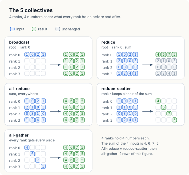
Five collectives cover most programs. We work each of them by hand on the same 4 ranks, each of which holds 4 numbers:
| Rank | Its data |
|---|---|
| 0 | 1, 0, 2, 1 |
| 1 | 2, 1, 0, 3 |
| 2 | 0, 3, 1, 0 |
| 3 | 1, 2, 4, 1 |
| element-by-element sum | 4, 6, 7, 5 |
Each element of the sum adds 1 number from every rank. For example, element 1 of the sum is 0 + 1 + 3 + 2 = 6, the element 1 of ranks 0, 1, 2 and 3.
Definition 28.5 Broadcast. In a broadcast, the root holds a buffer, and afterward every rank holds a copy of it.
Example. With rank 0 as the root, the 4 numbers 1, 0, 2, 1 of rank 0 are copied to ranks 1, 2 and 3. Afterward all 4 ranks hold 1, 0, 2, 1, and the former data of ranks 1, 2 and 3 is overwritten.
Definition 28.6 Reduce. In a reduce, every rank holds a buffer of the same length, and afterward the root holds the element-by-element combination of all the buffers. The other ranks receive nothing.
Example. With rank 0 as the root and the sum as the combination, rank 0 ends with 4, 6, 7, 5. Ranks 1, 2 and 3 still hold their own data.
Definition 28.7 All-reduce. In an all-reduce, every rank holds a buffer of the same length, and afterward every rank holds the element-by-element combination of all the buffers. An all-reduce has no root.
Example. All 4 ranks end with 4, 6, 7, 5. The gradients of Section 28.1.1 are combined in the same way, and there every rank ends with 6, 4, 4.
Definition 28.8 Reduce-scatter. In a reduce-scatter, every rank holds a buffer of the same length, which is divided into k pieces of equal length. Afterward rank r holds piece r of the combination, and only that piece.
Example. With 4 ranks and 4 numbers, each piece is 1 number. Rank 0 ends with 4, rank 1 with 6, rank 2 with 7 and rank 3 with 5. Rank 1, for instance, receives element 1 of the sum, 0 + 1 + 3 + 2 = 6.
Definition 28.9 All-gather. In an all-gather, rank r holds piece r of a buffer, and afterward every rank holds all k pieces, in the order of the ranks.
Example. Rank 0 holds 4, rank 1 holds 6, rank 2 holds 7 and rank 3 holds 5. Afterward every rank holds 4, 6, 7, 5.
Figure 28.1 shows the 5 collectives on these 4 ranks.
The following table summarizes the 5 definitions.
| Collective | Before | After |
|---|---|---|
| broadcast | the root holds the data | every rank holds a copy |
| reduce | every rank holds data | the root holds the combination |
| all-reduce | every rank holds data | every rank holds the combination |
| reduce-scatter | every rank holds data | rank r holds piece r of the combination |
| all-gather | rank r holds piece r | every rank holds all the pieces |
Data-parallel training needs an all-reduce, because every rank contributes a gradient and every rank needs the sum.
28.2.2 Reduction operators
So far the combination has always been the sum, but the definitions of reduce, all-reduce and reduce-scatter allow other ways of combining 2 numbers into 1.
Definition 28.10 Reduction operator. A reduction operator combines 2 numbers into 1 and is applied element by element, such as a sum, a product, a minimum or a maximum. The operator must be associative, that is, (a + b) + c = a + (b + c), because each algorithm groups the operations in its own order.
Example. An all-reduce of the 4 ranks above with the maximum as its operator gives every rank 2, 3, 4, 3. Element 0, for instance, is the largest of 1, 2, 0 and 1.
NCCL provides ncclSum, ncclProd, ncclMin, ncclMax and ncclAvg, the sum divided by the
number of ranks.
Recall from Chapter 8 that floating-point addition is associative only up to rounding. 2 algorithms that group the same additions differently can therefore return results that differ in the last bits. For this reason, the tests in this chapter use small whole numbers, whose sums are exact in any order, so that every rank’s result can be compared exactly with the expected sum.
28.2.3 Relations between collectives
The 5 collectives are related to each other. An all-reduce produces the same result as a reduce followed by a broadcast. It also produces the same result as a reduce-scatter followed by an all-gather. In Figure 28.1, the reduce-scatter leaves the sum 4, 6, 7, 5 spread over the 4 ranks, 1 number on each rank. The all-gather then gives every rank all 4 numbers, which is the result of the all-reduce.
The ring algorithm of Section 28.4 uses the second decomposition. Its first half makes each rank responsible for computing one piece of the sum, so the additions are divided evenly among the ranks. Its second half distributes the finished pieces to all ranks.
A program needs every rank to hold the maximum of 1 value per rank. Which collective is it, and with which operator?
An all-reduce with the maximum as its operator, ncclMax in NCCL. Every rank contributes 1 value
and every rank needs the result.
28.3 A cost model for messages
To compare algorithms, we need an estimate of the time that 1 message takes, where a message is the data that 1 rank sends to 1 other rank in 1 transfer. Let us first estimate 2 messages by hand over a link of 25 GB/s. A message of 100 MB occupies the link for 100 × 106 B ÷ (25 × 109 B/s) = 4 ms. By the same division, a message of 4 KB would occupy it for 0.16 µs. However, a message of any size must be started by the sender, must cross the link, and must be detected by the receiver, and these actions take microseconds regardless of the number of bytes. The time of a message therefore has two parts: a fixed part that every message pays, and a part that grows with the number of bytes.
In Section 4.3, we modeled a copy between the host and the device in exactly this way, as a fixed start-up time plus the number of bytes divided by the bandwidth. The same model applies to a message between 2 ranks:
\[ T = \alpha + \frac{m}{B} \]
| Symbol | Meaning | In the example |
|---|---|---|
| \(\alpha\) | latency of a message: the fixed time that every message costs, regardless of its size | 10 µs |
| \(m\) | the size of the message | 4 KB or 100 MB |
| \(B\) | the bandwidth of the link | 25 GB/s |
| \(T\) | the time of 1 message | 10.2 µs or 4.0 ms |
The latency \(\alpha\) includes everything that does not depend on the size of the message: starting the transfer, the time for the signal to cross the link, and the time for the receiver to detect that the data has arrived. Many texts write the second term as \(\beta m\), where \(\beta = 1 / B\) is the time per byte, and therefore call this model the α-β model. We keep the bandwidth \(B\), because link bandwidths are quoted in GB/s.
For example, over a link with α = 10 µs and B = 25 GB/s, a message of 4 KB takes 10 µs + 4,000 B ÷ (25 × 109 B/s) = 10 µs + 0.16 µs = 10.2 µs, of which the fixed time is 98%. A message of 100 MB takes 10 µs + 100 × 106 B ÷ (25 × 109 B/s) = 10 µs + 4,000 µs = 4.0 ms, of which the fixed time is 0.25%. The 2 parameters are round numbers of the same order as the copies measured in Chapter 4.
Small messages are therefore latency-bound: their time is approximately the number of messages that must be sent one after another, multiplied by \(\alpha\). Large messages are bandwidth-bound: their time is approximately the number of bytes on the busiest link divided by \(B\). It follows that a good algorithm for small messages sends few messages in sequence, whereas a good algorithm for large messages sends few bytes over each link. As we will see in the next 2 sections, the ring is the better algorithm for large messages and the tree is the better algorithm for small ones.
28.4 Ring all-reduce
28.4.1 Chunks and steps of the ring
Recall the problem of Section 28.1.2. With a single collector, the link of rank 0 carried every byte of the exchange, while the links of ranks 1, 2 and 3 were mostly idle. A remedy follows from Section 28.2.3. An all-reduce is a reduce-scatter followed by an all-gather, and in a reduce-scatter each rank computes only one piece of the sum. If each of 4 ranks is responsible for a quarter of the sum, all 4 links can share the traffic. The ring all-reduce organizes the ranks and their data so that this happens. We first define its 2 ingredients and then follow the data by hand.
Definition 28.11 Ring. In a ring, the k ranks are arranged in a circle. Rank r sends only to the next rank, (r + 1) mod k, and receives only from the previous rank, (r − 1) mod k.
Example. In a ring of 4 ranks, rank 0 sends to rank 1, rank 1 to rank 2, rank 2 to rank 3, and rank 3 to rank 0. Rank 0 receives from rank 3.
Definition 28.12 Chunk and step. The message of m bytes on each rank is divided into k equal chunks of m / k bytes, numbered 0 to k − 1. A step is a round in which every rank sends exactly 1 chunk to the next rank and receives exactly 1 chunk from the previous rank, all at the same time.
Example. With k = 4 ranks of 8 floats each, every rank holds 4 chunks of 2 floats. In 1 step, the 4 ranks send 4 chunks at once, 1 over each link of the ring.
The algorithm has 2 phases, which correspond to the 2 collectives of Section 28.2.3:
- Reduce-scatter, k − 1 steps. In each step, every rank sends 1 chunk to the next rank, which adds it to its own copy of that chunk. Each chunk travels around the ring and collects the contribution of 1 more rank in every step.
- All-gather, k − 1 steps. At the start of this phase, every rank holds 1 complete chunk. In each step, every rank sends 1 complete chunk to the next rank, which stores it in place of its own copy.
Before we write the algorithm down, let us follow 1 chunk by hand. Take 4 ranks, and let rank r hold the value r + 1 in every element: rank 0 holds 1, rank 1 holds 2, rank 2 holds 3 and rank 3 holds 4, so every element of the sum is 1 + 2 + 3 + 4 = 10. Chunk 0 starts its journey at rank 0. In step 1, rank 0 sends its chunk 0, which holds 1, to rank 1, and rank 1 adds its own 2. Chunk 0 of rank 1 now holds 3 = 1 + 2, the contributions of ranks 0 and 1. In step 2, rank 1 passes this 3 to rank 2, which adds its 3 and obtains 6, the contributions of ranks 0, 1 and 2. In step 3, rank 2 passes the 6 to rank 3, which adds its 4 and obtains 10. After 3 steps, chunk 0 of rank 3 contains the contribution of every rank.
The all-gather phase then copies this finished chunk forward. In step 4, rank 3 sends the 10 to rank 0; in step 5, rank 0 sends it to rank 1; and in step 6, rank 1 sends it to rank 2. Chunk 0 has moved 6 times, each time to the next rank, and every rank now holds 10 in chunk 0. Every other chunk follows the same path, but chunk c starts at rank c. In step 1, therefore, rank 0 sends chunk 0, rank 1 sends chunk 1, rank 2 sends chunk 2 and rank 3 sends chunk 3, and each of the 4 links carries exactly 1 chunk.
28.4.2 A ring all-reduce example
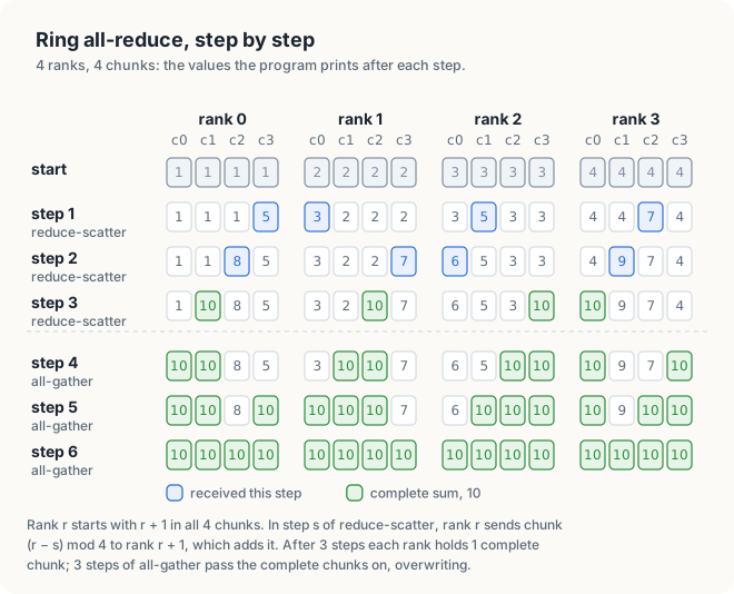
We now trace all 4 chunks together, for 4 ranks with 8 floats each, so that each chunk holds 2 floats. Rank r starts with r + 1 in every element, as above. The 2 floats of a chunk always hold the same value in this example, so the table shows 1 number per chunk, in the order chunk 0, chunk 1, chunk 2, chunk 3. In each row, the notation 0→1: c0 means that rank 0 sends chunk 0 to rank 1, and the chunk that changed on each rank is printed in bold.
Worked example: 4 ranks, 8 floats each, so 4 chunks of 2 floats
| After step | Transfers | Rank 0 | Rank 1 | Rank 2 | Rank 3 |
|---|---|---|---|---|---|
| start | 1 1 1 1 | 2 2 2 2 | 3 3 3 3 | 4 4 4 4 | |
| 1, reduce-scatter | 0→1: c0, 1→2: c1, 2→3: c2, 3→0: c3 | 1 1 1 5 | 3 2 2 2 | 3 5 3 3 | 4 4 7 4 |
| 2, reduce-scatter | 0→1: c3, 1→2: c0, 2→3: c1, 3→0: c2 | 1 1 8 5 | 3 2 2 7 | 6 5 3 3 | 4 9 7 4 |
| 3, reduce-scatter | 0→1: c2, 1→2: c3, 2→3: c0, 3→0: c1 | 1 10 8 5 | 3 2 10 7 | 6 5 3 10 | 10 9 7 4 |
| 4, all-gather | 0→1: c1, 1→2: c2, 2→3: c3, 3→0: c0 | 10 10 8 5 | 3 10 10 7 | 6 5 10 10 | 10 9 7 10 |
| 5, all-gather | 0→1: c0, 1→2: c1, 2→3: c2, 3→0: c3 | 10 10 8 10 | 10 10 10 7 | 6 10 10 10 | 10 9 10 10 |
| 6, all-gather | 0→1: c3, 1→2: c0, 2→3: c1, 3→0: c2 | 10 10 10 10 | 10 10 10 10 | 10 10 10 10 | 10 10 10 10 |
In steps 1 to 3 the receiver adds the arriving chunk to its own; in steps 4 to 6 it overwrites its own chunk with the arriving one.
Every number in the table is a sum of contributions from consecutive ranks of the ring. For example, the 5 in chunk 3 of rank 0 after step 1 is 4 + 1, from ranks 3 and 0. In step 2, rank 0 passes it to rank 1, which adds 2 and obtains 7, the contributions of ranks 3, 0 and 1. In step 3, rank 1 passes the 7 to rank 2, which adds 3 and obtains 10. After step 3, each rank holds exactly 1 complete chunk: rank 0 holds chunk 1, rank 1 chunk 2, rank 2 chunk 3 and rank 3 chunk 0, that is, rank r holds chunk (r + 1) mod 4. Steps 4 to 6 copy each of these 4 complete chunks 3 times around the ring.
Figure 28.2 shows the data of every rank after every step. These are also the values that the program of Section 28.6 prints when it runs this case.
Animation 1 shows the same 6 steps with the chunks in transit between the ranks.
Key observation In every step of the ring, every rank sends exactly 1 chunk and receives exactly 1 chunk. All k links therefore carry the same number of bytes at the same time, and no link waits while another one works, which is the property that the single collector of Section 28.1.2 lacked.
The following procedure describes the algorithm from the point of view of rank r. The array \(data\) holds the k chunks of the rank, and all rank and chunk numbers are taken modulo k, so the previous rank of rank 0 is rank k − 1.
Ring-All-Reduce(\(data, r, k\))
- for \(s \in [0, k-1)\) { // reduce-scatter
- send \(data[(r - s) \bmod k]\) to rank \((r + 1) \bmod k\)
- \(c = (r - 1 - s) \bmod k\)
- receive \(x\) from rank \((r - 1) \bmod k\)
- \(data[c] = data[c] + x\)
- }
- // now \(data[(r + 1) \bmod k]\) holds the complete sum
- for \(s \in [0, k-1)\) { // all-gather
- send \(data[(r + 1 - s) \bmod k]\) to rank \((r + 1) \bmod k\)
- \(c = (r - s) \bmod k\)
- receive \(x\) from rank \((r - 1) \bmod k\)
- \(data[c] = x\)
- }
Lines 1 to 6 are the reduce-scatter, and iteration s of the loop is step s + 1 of the table. In line 2, rank r sends the chunk to which it added in the previous step; in step 1, where s = 0, this is its own chunk r, which no other rank has touched yet. The previous rank follows the same rule, so the chunk that arrives is chunk (r − 1 − s) mod k, which line 3 computes. Line 5 adds the arriving partial sum to the rank’s own contribution. For rank 1 in step 1, line 2 sends chunk 1, line 3 gives c = 0, and line 5 computes 2 + 1 = 3, the bold 3 in the first row of the table. Lines 8 to 13 are the all-gather. They have the same form, but rank r starts by sending its complete chunk, (r + 1) mod k, and line 12 overwrites the chunk instead of adding to it.
The code does not make it obvious that every rank ends with the complete sum in every chunk, so we prove it. The proof follows the partial sums of the table: after each step of the reduce-scatter, the chunk that a rank has just received contains the contributions of 1 more rank.
Theorem 28.1 Let the k ranks run Ring-All-Reduce. After step t of the reduce-scatter, for t = 1, …, k − 1, chunk (r − t) mod k of rank r holds the sum of the contributions of the t + 1 ranks r − t, r − t + 1, …, r, taken modulo k. When the procedure ends, every chunk of every rank holds the sum of the contributions of all k ranks.
For instance, after step 2 the table shows 7 in chunk (1 − 2) mod 4 = 3 of rank 1, and 7 = 4 + 1 + 2 are the contributions of ranks 3, 0 and 1.
Proof. Reduce-scatter, step 1. In step 1, s = 0, and rank r receives chunk (r − 1) mod k from rank r − 1. Rank r − 1 sends its own chunk r − 1 in line 2, and that chunk still holds only the contribution of rank r − 1. Line 5 adds the contribution of rank r. Chunk r − 1 of rank r therefore holds the contributions of ranks r − 1 and r, which is the claim for t = 1.
Reduce-scatter, step t + 1. Assume the claim after step t, where 1 ≤ t < k − 1. In step t + 1, s = t, and rank r receives chunk (r − 1 − t) mod k from rank r − 1. By the assumption applied to rank r − 1, this chunk holds the contributions of the t + 1 ranks r − 1 − t, …, r − 1. Rank r’s own copy of the chunk still holds only rank r’s contribution, because in steps 1 to t rank r changed only chunks r − 1, r − 2, …, r − t, and since t + 1 < k, chunk r − 1 − t is none of them. After line 5, chunk r − (t + 1) of rank r holds the contributions of the t + 2 ranks r − (t + 1), …, r, which is the claim for t + 1.
End of the reduce-scatter. After step k − 1, chunk (r − (k − 1)) mod k = (r + 1) mod k of rank r holds the contributions of k consecutive ranks of the ring, which are all k ranks, as line 7 states.
All-gather. We show that after t steps of the all-gather, rank r holds the complete sum in the t + 1 chunks (r + 1 − j) mod k for j = 0, …, t. For t = 0, this is the previous paragraph. In step t + 1, s = t, and rank r receives chunk (r − t) mod k from rank r − 1, which sends its chunk ((r − 1) + 1 − t) mod k = (r − t) mod k in line 9. By the assumption applied to rank r − 1, that chunk is complete, and line 12 copies it. Rank r thus gains the complete chunk r + 1 − (t + 1). After k − 1 steps, rank r holds the complete sum in the k chunks (r + 1 − j) mod k, j = 0, …, k − 1, which are all of its chunks. ∎
28.4.3 Steps and bytes of the ring
Let us first count the traffic of the example of Section 28.4.2. Each rank sends 1 chunk of 2 floats in each of 6 steps, 12 floats in all, and it receives the same 12 floats. The message on each rank is 8 floats, so each rank sends 12 ÷ 8 = 1.5 times its message.
Now count the collector of Section 28.1.2 on the same data. Ranks 1, 2 and 3 each send their 8 floats to rank 0, so 24 floats enter the link of rank 0. Rank 0 then sends the sum of 8 floats to each of the 3 other ranks, so 24 floats leave through the same link. The link of rank 0 thus carries 24 floats in each direction, twice the 12 floats of any link of the ring. Moreover, the collector cannot send the sum before it has received all 3 messages, so its two directions work one after the other: the exchange lasts as long as 24 + 24 = 48 floats crossing 1 link. In the ring, every link sends and receives its 12 floats at the same time, so the exchange lasts as long as 12 floats crossing 1 link. The ring is 48 ÷ 12 = 4 times as fast, a factor of k, as we show in Section 28.4.4 in general.
For k ranks and a message of m bytes, each phase of the ring takes k − 1 steps, so the all-reduce takes 2 (k − 1) steps. In each step, a rank sends 1 chunk of m / k bytes. Over the whole all-reduce, each rank therefore sends
\[ 2 (k - 1) \cdot \frac{m}{k} = \frac{2 (k - 1)}{k} \, m \]
bytes, and it receives the same number of bytes. For k = 4, the factor is 2 × 3 / 4 = 1.5, as counted above.
The factor 2 (k − 1) / k approaches 2 as the number of ranks grows. It is 1.5 for 4 ranks, 1.75 for 8 ranks and 1.97 for 64 ranks. The number of bytes on each link therefore barely grows with the number of ranks.
An argument from the 2 phases shows why no algorithm can do much better. In a reduce-scatter, each rank holds its contribution to the k − 1 pieces that other ranks finish, (k − 1) m / k bytes, and no other rank holds these bytes, so each rank must send at least (k − 1) m / k bytes. In an all-gather, each rank must receive the (k − 1) m / k bytes of the pieces that it did not finish. Every byte that is received was sent by some rank, so the k ranks together send at least k × (k − 1) m / k bytes, on average (k − 1) m / k per rank. Over the 2 phases, some rank must therefore send at least 2 (k − 1) m / k bytes. Patarasuk and Yuan proved in 2009 that the same bound holds for any all-reduce algorithm, not only for those built from these 2 phases: some rank must send at least 2 (k − 1) / k of the message over its link. The ring reaches this lower bound, so it is said to be bandwidth-optimal.
With the cost model of Section 28.3, the time of a ring all-reduce is
\[ T_{\text{ring}} = 2 (k - 1) \, \alpha + \frac{2 (k - 1)}{k} \cdot \frac{m}{B} \]
| Symbol | Meaning | For the example of section 28.1.2 |
|---|---|---|
| \(k\) | number of ranks | 4 |
| \(m\) | message per rank | 100 MB |
| \(2 (k - 1)\) | number of steps, each costing \(\alpha\) | 6 |
| \(2 (k - 1) m / k\) | bytes that each link carries in each direction | 150 MB |
| \(T_{\text{ring}}\) | the time, with α = 10 µs and B = 25 GB/s | 0.06 ms + 6 ms |
28.4.4 Comparison with a single collecting rank
Figure 28.3 compares the ring with the collector of Section 28.1.2, for the same 4 ranks, 100 MB and links of 25 GB/s. The link of the collector carries 300 MB in each direction, which takes 24 ms. Each link of the ring carries 2 × 3 / 4 × 100 MB = 150 MB in each direction, and all the links work at the same time, so the exchange takes 6 ms.
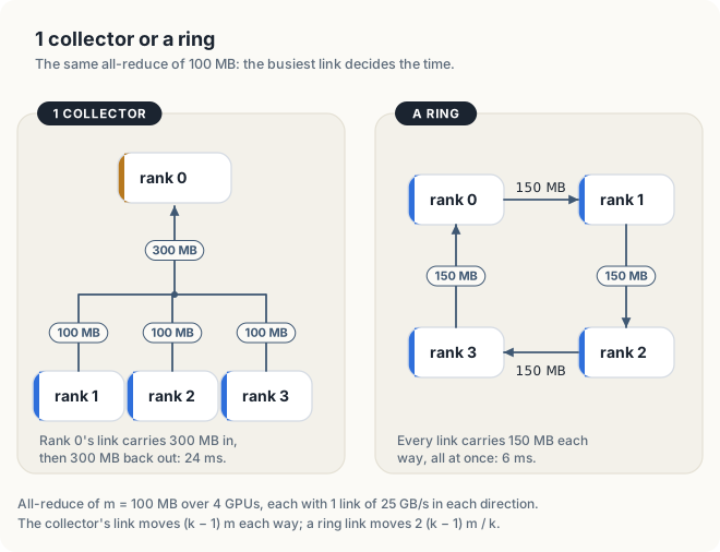
In general, the ratio between the 2 times is k. The link of the collector moves 2 (k − 1) m bytes, whereas each link of the ring moves 2 (k − 1) m / k bytes. For 8 ranks the ring is therefore 8 times as fast, and for 64 ranks 64 times as fast. The cost of the ring is its number of steps, 2 (k − 1), each of which pays α. For a large message, the fixed time of 6 × 10 µs = 60 µs is 1% of the 6 ms total. For a small message, however, the fixed time is nearly all of the total.
For large messages, the bandwidth term determines how long an all-reduce takes on real hardware. The following table assumes 8 GPUs in a ring and a gradient of 1 GB, the 250 million parameters of Section 28.1.1. It gives the bandwidth term, 1.75 × 1 GB ÷ B, at the rated bandwidth of each kind of link in 1 direction. Measured transfers reach less than the rated bandwidth, as we found for PCIe in Chapter 4.
| Link between GPUs | Rated bandwidth, 1 direction | 1.75 GB at that rate |
|---|---|---|
| PCIe 4.0 × 16 (RTX 4090, A100 PCIe) | 32 GB/s | 55 ms |
| PCIe 5.0 × 16 (RTX 5090, H100 PCIe) | 63 GB/s | 28 ms |
| InfiniBand NDR, 400 Gb/s (between servers) | 50 GB/s | 35 ms |
| NVLink 3, A100 SXM (12 links) | 300 GB/s | 5.8 ms |
| NVLink 4, H100 SXM (18 links) | 450 GB/s | 3.9 ms |
| NVLink 5, B200 (18 links) | 900 GB/s | 1.9 ms |
Note that NVIDIA quotes NVLink bandwidth as the total of both directions, 600, 900 and 1,800 GB/s for the 3 generations; the table gives half of each figure. SXM denotes the module form of a data-center GPU, which is mounted on a server board, as opposed to a PCIe card, and NDR is the 400 Gb/s generation of InfiniBand, a network that connects servers. A machine with only 1 GPU, such as a single DGX Spark, has no link between GPUs.
In a ring all-reduce, each link carries 2 (k − 1) / k of the message, which is less than twice the message for any number of ranks.
28.5 Tree all-reduce
28.5.1 Binomial trees
The ring needs 2 (k − 1) steps, and each step pays the latency α. For 1,024 ranks, this is 2,046 steps. A tree needs far fewer steps, because in each step it halves the number of ranks that still hold a partial sum, instead of adding 1 contribution at a time.
Let us first work a tree by hand on 4 ranks that hold 1, 2, 3 and 4, so that the sum is 10. In step 1, rank 1 sends its 2 to rank 0, which now holds 1 + 2 = 3, and at the same time rank 3 sends its 4 to rank 2, which now holds 3 + 4 = 7. Two partial sums remain, on ranks 0 and 2. In step 2, rank 2 sends its 7 to rank 0, which now holds 3 + 7 = 10, the complete sum. Two steps have reduced 4 contributions to 1. The broadcast repeats the same pairs in the opposite order and direction. In step 3, rank 0 sends 10 to rank 2. In step 4, rank 0 sends 10 to rank 1 and, at the same time, rank 2 sends 10 to rank 3. After 4 steps, every rank holds 10, whereas the ring of Section 28.4.2 needed 6 steps for the same 4 ranks.
The tree pays for its fewer steps with larger messages. In this example, rank 0 received the whole message in steps 1 and 2 and sent the whole message in steps 3 and 4, so its link carried 2 whole messages in each direction, compared with 1.5 messages for a link of the ring.
Definition 28.13 Binomial tree. For k ranks, where k is a power of 2, a binomial tree pairs up the ranks at a distance of 1, then pairs up the receivers at a distance of 2, then at a distance of 4, and so on, so it has log2 k levels. In each pair, the rank with the higher number sends to the rank with the lower number.
Example. For k = 4, the pairs of level 1 are ranks 1 → 0 and 3 → 2, and the pair of level 2 is rank 2 → 0. The tree has log2 4 = 2 levels.
A tree all-reduce has 2 phases:
- Reduce up the tree, log2 k steps. In step 1, every odd rank sends its whole message to the even rank below it, which adds it to its own data. In step 2, the receivers of step 1 pair up at a distance of 2, then at a distance of 4, and so on, until rank 0 holds the sum of all the messages.
- Broadcast down the tree, log2 k steps. The same pairs are used in the opposite order and direction: rank 0 sends the total to rank k / 2, then both of them send it on, and so on.
The following procedure describes the algorithm from the point of view of rank r. The variable \(d\) is the distance between the 2 ranks of a pair, and \(data\) is the whole message of the rank.
Tree-All-Reduce(\(data, r, k\))
- \(d = 1\) // k is a power of 2
- while \(d < k\) { // reduce: log2 k steps
- if \(r \bmod 2d = d\), send \(data\) to rank \(r - d\)
- if \(r \bmod 2d = 0\), receive \(x\) from rank \(r + d\) and set \(data = data + x\)
- \(d = 2d\)
- }
- \(d = k / 2\)
- while \(d \ge 1\) { // broadcast: log2 k steps
- if \(r \bmod 2d = 0\), send \(data\) to rank \(r + d\)
- if \(r \bmod 2d = d\), receive \(x\) from rank \(r - d\) and set \(data = x\)
- \(d = d / 2\)
- }
Lines 2 to 6 are the reduce phase. With d = 1, line 3 selects the odd ranks as senders and line 4 the even ranks as receivers, as in step 1 of the example. With d = 2, only ranks whose number is a multiple of 2 take part: rank 2 sends and rank 0 receives. A rank that has sent its data takes no further part in the reduce phase, because its number fails both tests for every larger d. Lines 8 to 12 are the broadcast phase, which uses the same pairs with d halving, and line 10 overwrites instead of adding.
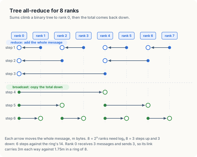
Figure 28.4 shows the tree for k = 8. The all-reduce takes 2 × log2 8 = 6 steps, compared with 2 × 7 = 14 steps for a ring of 8 ranks. However, every arrow in the tree carries the whole message of m bytes, because the message is not divided into chunks. Rank 0 receives a message in each of the 3 steps of the reduce phase and sends a message in each of the 3 steps of the broadcast phase, so its link carries 3m in each direction, compared with 1.75m for a ring of 8 ranks. The time of the tree all-reduce is therefore
\[ T_{\text{tree}} = 2 \log_2 k \, \left( \alpha + \frac{m}{B} \right) \]
Compared with the ring, the number of steps contains \(\log_2 k\) in place of \(k - 1\), and every step carries the whole message rather than a chunk.
Key observation The ring divides the message into k chunks and sends 1 chunk per step in 2 (k − 1) steps; the tree sends the whole message in each of 2 log2 k steps. The ring therefore pays more fixed time α, and the tree more time per byte.
28.5.2 Choosing between the ring and the tree
Having derived the time of both algorithms, we can now determine which one is faster for a given message size. For k = 8, the 2 formulas are
\[ T_{\text{ring}} = 14 \alpha + 1.75 \frac{m}{B} \qquad T_{\text{tree}} = 6 \alpha + 6 \frac{m}{B} \]
The tree saves 8α of fixed time but carries 4.25 m / B more traffic. The 2 times are equal when 8α = 4.25 m / B, which happens at the crossover size
\[ m^{\ast} = \frac{8 \alpha B}{4.25} \]
Worked example: the crossover for α = 10 µs, B = 25 GB/s, k = 8
- 8α = 80 µs, the fixed time that the tree saves.
- m* = 80 × 10−6 s × 25 × 109 B/s ÷ 4.25 = 2,000,000 B ÷ 4.25 = 470,588 bytes, about 470 KB.
- Check: the ring takes 140 µs + 1.75 × 470,588 B ÷ 25 GB/s = 140 µs + 33 µs = 173 µs. The tree takes 6 × (10 µs + 18.8 µs) = 173 µs.
Below 470 KB the tree is faster, and above 470 KB the ring is faster. Figure 28.5 plots both formulas for messages from 1 KB to 1 GB. For a message of 4 KB, the tree takes 60 µs and the ring 140 µs. For a message of 1 GB, the ring takes 70 ms and the tree 240 ms.
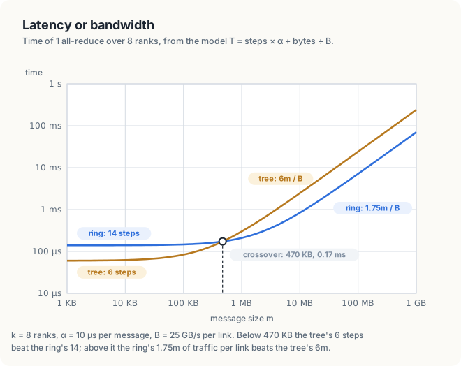
A gradient of 1 GB is far above the crossover, which is why rings carry most of the traffic of data-parallel training. Small all-reduces, such as the reduction of a single loss value or of a flag that indicates whether training should stop, are far below it.
NCCL improves on both of these simple algorithms. Since version 2.4, it uses a double binary tree: 2 trees over the same ranks, each of which carries half of the data. A rank that is a leaf in one tree is an inner node in the other, so no rank performs the work of an inner node twice. In addition, the message is divided into small pieces that follow each other through the tree. This pipelining keeps every level of the tree busy at the same time. The result keeps the logarithmic number of steps of the tree and comes close to the bandwidth of the ring. NCCL chooses the ring, the tree or another algorithm for each call, based on the message size, the number of ranks and the topology, the way in which the GPUs are connected to each other.
For k = 64 and the same α and B, does the crossover move up or down?
Up. The ring takes 126α + 1.97 m / B, the binomial tree 12α + 12 m / B. They meet at 114α = 10.03 m / B, so m* = 114 × 10 µs × 25 GB/s ÷ 10.03 = 2.8 MB. More ranks mean many more ring steps, so the tree remains faster up to larger messages.
28.6 Simulating collectives on 1 GPU
28.6.1 Ranks as slices of a buffer
We now implement both algorithms. The program of this section runs them on 1 GPU by placing all k ranks in the memory of that GPU, as k slices of 1 buffer. Rank r owns the floats from r n to r n + n − 1, where n is the number of floats per rank. A send from rank r to rank r + 1 then becomes a read from 1 slice and a write into another.
The program measures the algorithms, not a network. All the simulated links share the memory of 1 GPU, so the transfers of 1 step do not each have a link of their own. In Section 28.6.4, we show how this affects the measured times.
The program first converts an algorithm into a plan: a list of steps, each of which is a list of
transfers that run at the same time. A transfer specifies the offset that it reads from and the
offset that it writes to, and its step specifies whether the transfer adds to the destination or
overwrites it. Listing 28.1 shows the data structures. The function addStep appends the
transfers of 1 step to the plan and records where they start, how many there are, how many floats
each one moves, and whether they add.
Listing 28.1 A plan of steps and transfers. Rust C++
/// 1 step of a collective: `count` transfers of `len` floats that run at the same time.
struct Step {
    first: usize,
    count: usize,
    len: usize,
    add: bool,
}

/// The (from, to) offsets of every transfer, and the steps that group them.
#[derive(Default)]
struct Plan {
    pairs: Vec<u32>,
    steps: Vec<Step>,
}

impl Plan {
    fn add_step(&mut self, sends: &[(usize, usize)], len: usize, add: bool) {
        let first = self.pairs.len() / 2;

        for &(from, to) in sends {
            self.pairs.push(from as u32);
            self.pairs.push(to as u32);
        }
        self.steps.push(Step { first, count: sends.len(), len, add });
    }
    // ...
}
// 1 send: `len` floats from offset `from` of the buffer to offset `to`.
struct Transfer {
int from;
int to;
};
// 1 step of a collective: transfers that run at the same time, on different links.
struct Step {
int first; // index of the step's first transfer in the plan
int count; // number of transfers
int len; // floats per transfer
bool add; // add into the destination, or overwrite it
};
struct Plan {
std::vector<Transfer> transfers;
std::vector<Step> steps;
};
void addStep(Plan& plan, const std::vector<Transfer>& sends, int len, bool add)
{
int first = int(plan.transfers.size());
plan.transfers.insert(plan.transfers.end(), sends.begin(), sends.end());
plan.steps.push_back({first, int(sends.size()), len, add});
}
The Rust version stores each transfer as 2 numbers in 1 flat Vec<u32>, so that the plan
can be copied to the GPU with DeviceBuffer::from_host and read by the kernel as a &[u32].
The function ring in Listing 28.2 builds the plan of the procedure Ring-All-Reduce of Section
28.4.2. The first loop creates the k − 1 reduce-scatter steps of lines 1 to 6. In step s, rank r
sends its chunk (r − s) mod k to rank (r + 1) % k, and the step adds. The second loop creates
the k − 1 all-gather steps, in which rank r sends its chunk (r + 1 − s) mod k, and the step
overwrites. The term + k inside each % keeps the left operand positive, because the % of a
negative int is negative in C++. The function tree builds the 2 phases of Section 28.5.1 in the
same way, with the distance d doubling in the reduce phase and halving in the broadcast phase.
Listing 28.2 The ring and the tree as plans.
/// Ring: reduce-scatter in k - 1 steps, then all-gather in k - 1 steps.
fn ring(k: usize, n: usize) -> Plan {
let mut plan = Plan::default();
let chunk = n / k;
let send = |r: usize, c: usize| (r * n + c * chunk, (r + 1) % k * n + c * chunk);
for s in 0..k - 1 {
let sends: Vec<_> = (0..k).map(|r| send(r, (r + k - s) % k)).collect();
plan.add_step(&sends, chunk, true);
}
for s in 0..k - 1 {
let sends: Vec<_> = (0..k).map(|r| send(r, (r + 1 + k - s) % k)).collect();
plan.add_step(&sends, chunk, false);
}
plan
}
/// Binomial tree, k a power of 2: sums climb to rank 0, then the total comes back down.
fn tree(k: usize, n: usize) -> Plan {
let mut plan = Plan::default();
let mut d = 1;
while d < k {
let sends: Vec<_> = (d..k).step_by(2 * d).map(|r| (r * n, (r - d) * n)).collect();
plan.add_step(&sends, n, true);
d *= 2;
}
d = k / 2;
while d >= 1 {
let sends: Vec<_> = (0..k).step_by(2 * d).map(|r| (r * n, (r + d) * n)).collect();
plan.add_step(&sends, n, false);
d /= 2;
}
plan
}// Ring: reduce-scatter in k - 1 steps, then all-gather in k - 1 steps.
// Rank r owns elements [r n, r n + n) of the buffer; chunk c is n / k floats.
Plan ring(int k, int n)
{
Plan plan;
int chunk = n / k;
for (int s = 0; s < k - 1; ++s) {
std::vector<Transfer> sends;
for (int r = 0; r < k; ++r) {
int c = (r - s + k) % k;
int next = (r + 1) % k;
sends.push_back({r * n + c * chunk, next * n + c * chunk});
}
addStep(plan, sends, chunk, true);
}
for (int s = 0; s < k - 1; ++s) {
std::vector<Transfer> sends;
for (int r = 0; r < k; ++r) {
int c = (r + 1 - s + k) % k;
int next = (r + 1) % k;
sends.push_back({r * n + c * chunk, next * n + c * chunk});
}
addStep(plan, sends, chunk, false);
}
return plan;
}
// Binomial tree, k a power of 2: sums climb to rank 0, then the total comes back down.
Plan tree(int k, int n)
{
Plan plan;
for (int d = 1; d < k; d *= 2) {
std::vector<Transfer> sends;
for (int r = d; r < k; r += 2 * d) {
sends.push_back({r * n, (r - d) * n});
}
addStep(plan, sends, n, true);
}
for (int d = k / 2; d >= 1; d /= 2) {
std::vector<Transfer> sends;
for (int r = 0; r < k; r += 2 * d) {
sends.push_back({r * n, (r + d) * n});
}
addStep(plan, sends, n, false);
}
return plan;
}
28.6.2 The step kernel
Each step of a plan runs as 1 launch of 1 kernel, the function that runs on the GPU. All the
transfers of a step share the launch. If a step has count transfers and each transfer is given
per blocks, block b works on transfer b / per, and the per blocks of a transfer stride
through its floats together. Figure 28.6 shows step one of the ring for 4 ranks.
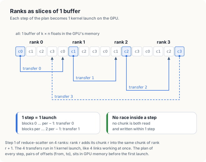
Running all the transfers of a step in 1 launch is correct only if no transfer reads an element
that another transfer of the same step writes. Both algorithms satisfy this condition. In
reduce-scatter step s of the ring, rank r + 1 receives chunk (r − s) and sends chunk
(r + 1 − s), which are 2 different chunks. In a step of the tree, the ranks that send and the ranks
that receive are 2 separate sets. The order of the steps is maintained by the stream, the
queue of GPU work introduced in Chapter 6: a launch starts only after the previous launch on the
same stream has finished.
In the kernel runStep of Listing 28.3, each thread first reads the transfer of its block,
sends[blockIdx.x / per]. The loop then starts at the thread’s position within the per blocks
of the transfer and advances by stride, the total number of threads that work on the transfer.
In each iteration, the thread reads 1 float from the source slice and either adds it to the
destination or overwrites the destination, depending on add. The host function run computes
per and launches the kernel on the stream.
Listing 28.3 The step kernel and its launch.
mod kernels {
// ...
/// `per` blocks for each transfer of the step; block b works on transfer b / per.
/// `plan` holds (from, to) offset pairs; the step's pairs start at pair `first`.
#[kernel]
#[launch_contract(domain = 1, block = (256, 1, 1))]
pub fn step(
mut all: DisjointSlice<f32>,
plan: &[u32],
first: u32,
len: u32,
per: u32,
add: u32,
) {
let b = thread::blockIdx_x();
let t = (first + b / per) as usize;
let from = plan[2 * t];
let to = plan[2 * t + 1];
let stride = per * BLOCK;
let mut i = (b % per) * BLOCK + thread::threadIdx_x();
while i < len {
// SAFETY: within 1 step no element is both read and written, and no 2
// threads write the same element, so these accesses cannot race.
unsafe {
let v = *all.get_unchecked_mut((from + i) as usize);
let d = all.get_unchecked_mut((to + i) as usize);
*d = if add != 0 { *d + v } else { v };
}
i += stride;
}
}
// ...
}
impl Gpu<'_> {
// ...
fn run(&mut self, steps: &[Step], pairs: &DeviceBuffer<u32>) -> Result<(), Error> {
for st in steps {
let per = st.len.div_ceil(BLOCK as usize).min((1024 / st.count).max(1)) as u32;
let config = LaunchConfig1D::new(st.count as u32 * per, BLOCK, 0);
let launch = self.module.prepare_step(config)?;
let (first, len, add) = (st.first as u32, st.len as u32, st.add as u32);
let all = &mut self.all;
self.module.step(self.stream, &launch, all, pairs, first, len, per, add)?;
}
Ok(())
}
// ...
}// `per` blocks for each transfer of the step; block b works on transfer b / per.
// Within 1 step no element is both read and written, so the transfers cannot race.
__global__ void runStep(float* all, const Transfer* sends, int len, int per, bool add)
{
Transfer t = sends[blockIdx.x / per];
int stride = per * blockDim.x;
for (int i = (blockIdx.x % per) * blockDim.x + threadIdx.x; i < len; i += stride) {
float v = all[t.from + i];
all[t.to + i] = add ? all[t.to + i] + v : v;
}
}
void run(const Gpu& gpu, const Step& st, cudaStream_t s)
{
int per = std::min((st.len + 255) / 256, std::max(1024 / st.count, 1));
const Transfer* sends = gpu.sends + st.first;
runStep<<<st.count * per, 256, 0, s>>>(gpu.all, sends, st.len, per, st.add);
}
The function run gives every step at most 1,024 blocks of 256 threads, divided among its
transfers, and never gives a transfer more blocks than it has floats to cover. For example, a tree
step with 1 transfer of 4 Mi floats receives all 1,024 blocks, whereas a ring step with 8
transfers receives 128 blocks for each transfer.
In Rust, 2 threads may write to the same DisjointSlice only at indices that the compiler can
prove to be different, which is the thread’s own index. The step kernel writes at to + i and
reads at from + i, where the offsets come from the plan, so it uses get_unchecked_mut inside an
unsafe block, as the per-block writes of Chapter 8 did. The SAFETY comment states the argument
of the previous paragraph. No element is both read and written within 1 step.
28.6.3 Running the 4-rank example
The measurements in this section come from a Jetson Orin NX, an integrated GPU with 8 SMs (streaming multiprocessors) and 102 GB/s of memory bandwidth. The program first runs the example of Section 28.4.2, 4 ranks of 8 floats, 1 step at a time, and prints the data of every rank after every step.
$ nvcc -arch=native allreduce.cu -o allreduce && ./allreduce
GPU: Orin, 8 SMs
ring all-reduce, 4 ranks of 8 floats: rank r starts with r + 1
rank 0 1 1 1 1 1 1 1 1
rank 1 2 2 2 2 2 2 2 2
rank 2 3 3 3 3 3 3 3 3
rank 3 4 4 4 4 4 4 4 4
after step 1 (reduce-scatter)
rank 0 1 1 1 1 1 1 5 5
rank 1 3 3 2 2 2 2 2 2
rank 2 3 3 5 5 3 3 3 3
rank 3 4 4 4 4 7 7 4 4
after step 2 (reduce-scatter)
rank 0 1 1 1 1 8 8 5 5
rank 1 3 3 2 2 2 2 7 7
rank 2 6 6 5 5 3 3 3 3
rank 3 4 4 9 9 7 7 4 4
after step 3 (reduce-scatter)
rank 0 1 1 10 10 8 8 5 5
rank 1 3 3 2 2 10 10 7 7
rank 2 6 6 5 5 3 3 10 10
rank 3 10 10 9 9 7 7 4 4
after step 4 (all-gather)
rank 0 10 10 10 10 8 8 5 5
rank 1 3 3 10 10 10 10 7 7
rank 2 6 6 5 5 10 10 10 10
rank 3 10 10 9 9 7 7 10 10
after step 5 (all-gather)
rank 0 10 10 10 10 8 8 10 10
rank 1 10 10 10 10 10 10 7 7
rank 2 6 6 10 10 10 10 10 10
rank 3 10 10 9 9 10 10 10 10
after step 6 (all-gather)
rank 0 10 10 10 10 10 10 10 10
rank 1 10 10 10 10 10 10 10 10
rank 2 10 10 10 10 10 10 10 10
rank 3 10 10 10 10 10 10 10 10
Each pair of columns is 1 chunk of 2 floats. The rows agree with the steps that we traced by hand in Section 28.4.2. After step 1, chunk 0 of rank 1 is 3 and chunk 3 of rank 0 is 5. After step 3, each rank holds 1 complete chunk of 10, and after step 6 all 32 floats are 10. The Rust program prints the same 35 lines.
28.6.4 Timing the ring and the tree
The program then runs both algorithms on 8 simulated ranks, for messages of 4 KiB, 64 KiB, 1 MiB
and 16 MiB per rank. For each size, it times 50 all-reduces with CUDA events (Chapter 6), each
starting from fresh values, and compares every element of every rank with the exact sum. Element
i of rank r starts as i % 16 + r, a whole number below 24, so the sum over 8 ranks is exact in
any order.
all-reduce on 8 simulated ranks
steps busiest rank sends
ring 14 1.75 x the message
tree 6 3.00 x the message
message ring tree
4 KiB 0.162 ms 0.070 ms
64 KiB 0.226 ms 0.143 ms
1024 KiB 0.913 ms 0.795 ms
16384 KiB 7.184 ms 6.645 ms
every rank holds the exact sum: PASSED
$ cargo oxide run
...
message ring tree
4 KiB 0.166 ms 0.073 ms
64 KiB 0.221 ms 0.129 ms
1024 KiB 1.082 ms 1.065 ms
16384 KiB 7.295 ms 6.655 ms
every rank holds the exact sum: PASSED
The first table confirms the counts of Sections 28.4.3 and 28.5.1: 14 and 6 steps, and 1.75 and 3 times the message through the busiest rank. Repeated runs differ by up to 25% at 1 MiB.
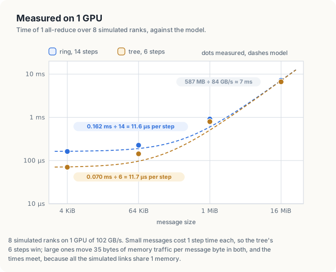
For small messages, the time follows the number of steps. At 4 KiB, the ring took 0.162 ms for 14 steps, 11.6 µs per step, and the tree took 0.070 ms for 6 steps, 11.7 µs per step. The tree was 0.162 ÷ 0.070 = 2.3 times as fast, which is the ratio of the step counts, 14 ÷ 6 = 2.3. On this GPU, the α of a step is therefore about 12 µs. A timeline from Nsight Systems (Chapter 25) divides it into about 9 µs inside the step kernel and 3.5 µs between 1 kernel and the next.
For large messages, the time follows the memory traffic. At 16 MiB, the two algorithms took about the same time, 7.2 ms and 6.6 ms. The reason is that the simulated links share 1 memory. A float that is added costs 12 bytes of memory traffic, 2 reads and 1 write, and a float that is copied costs 8 bytes, 1 read and 1 write. Both algorithms add (k − 1) n floats and copy (k − 1) n floats. For 16 MiB per rank, n = 16 MiB ÷ 4 bytes = 4,194,304 floats. The additions move 7 × 4,194,304 × 12 B = 352.3 MB and the copies 7 × 4,194,304 × 8 B = 234.9 MB, 587.2 MB in all, in the ring and in the tree alike. This is 35 bytes of memory traffic for every byte of the message. The ring took 7.184 ms, of which 0.162 ms was fixed time, so the memory moved 587.2 MB ÷ 7.022 ms = 84 GB/s, 82% of the GPU’s 102 GB/s.
The dashed lines of Figure 28.7 show the model T = steps × 11.6 µs + 35 m ÷ 84 GB/s. The model matches both ends of the measurements. At 1 MiB, where neither term dominates, the measured times lie about 0.3 ms above it.
On a machine with separate links, the two algorithms would differ at large sizes. A link of the ring would carry 1.75 × 16 MiB, whereas the link of the root of the tree would carry 3 × 16 MiB, so the ring would take about 1.75 ÷ 3 = 58% of the time of the tree. The simulation cannot show this difference, because its 8 links are 1 memory and only the total traffic matters. A simulation on 1 GPU therefore verifies the algorithm and measures the cost of its steps, but measuring the links requires 2 or more GPUs.
28.7 NCCL
28.7.1 Overview of NCCL
NCCL, the NVIDIA Collective Communications Library (pronounced “nickel”), implements the collectives of Section 28.2, as well as point-to-point sends and receives, for NVIDIA GPUs. It is open source, under a BSD license, and every major deep-learning framework uses it.
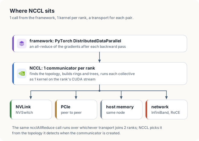
When a group of ranks starts, NCCL discovers the topology of the system: which GPUs share NVLink or an NVSwitch, which GPUs are under the same PCIe switch, and which GPUs are in other servers. From the topology, it builds rings and trees that use the fastest paths. For each pair of ranks, it chooses a transport, the path that the data takes. Within a server, it prefers peer-to-peer access over NVLink or PCIe, in which 1 GPU reads and writes the memory of another GPU directly. Where peer-to-peer access is not possible, it passes the data through a buffer in host memory. Between servers, it uses the network: InfiniBand, RoCE (remote memory access over Ethernet) or TCP sockets, the ordinary network connections of the operating system.
Each collective runs as 1 CUDA kernel on each rank, launched on a stream that the program chooses. The threads of the kernel move the data and perform the additions. They keep the steps of the algorithm in order through flags in memory, which the threads of 1 rank write and the threads of the next rank wait for. Unlike the simulation of Section 28.6, which launched 1 kernel per step, no host thread takes part between the steps. Figure 28.8 shows where NCCL sits between a framework and the hardware.
28.7.2 Communicators and the unique ID
Recall from Definition 28.3 that a communicator represents the membership of a rank in a group. In
NCCL, a communicator has the type ncclComm_t. It holds the size of the group, the number of the
rank within it, and the rings and connections that NCCL built for the group. Every collective takes
a communicator as a parameter.
Before ranks in different processes can communicate, they must agree that they belong to the same
group. One rank calls ncclGetUniqueId, which returns a ncclUniqueId, 128 bytes that identify the
group. The program sends these 128 bytes to every other rank through a channel of its own choice,
such as a file, a TCP connection, or a broadcast of MPI, the Message Passing Interface used in
supercomputer programs. Then, every rank calls ncclCommInitRank with the size of the group, the
ID and its own rank number. The following code shows these calls:
ncclUniqueId id;
if (rank == 0) check(ncclGetUniqueId(&id));
// send `id` to every rank, for example with MPI_Bcast
ncclComm_t comm;
check(cudaSetDevice(localGpu));
check(ncclCommInitRank(&comm, nranks, id, rank));
cuda-oxide does not wrap NCCL, so a Rust program makes these calls through other bindings to
the library, such as the nccl module of the cudarc crate, where Id::new and
Comm::from_rank correspond to the 2 calls above.
Rank 0 creates the ID in the second line, and every rank creates its communicator in the last line,
after selecting its GPU with cudaSetDevice. Note that ncclCommInitRank returns only when all
nranks ranks have called it with the same ID. A rank that never calls it, or that received a
different ID, leaves the other ranks waiting, which is the most common cause of hangs in multi-GPU
programs.
A single process that drives every GPU of 1 server does not need the ID. It can call
ncclCommInitAll, which creates k communicators at once, 1 for each device in a list.
28.7.3 Collectives on a stream
Once the communicator exists, an all-reduce is a single call:
check(ncclAllReduce(send, recv, count, ncclFloat, ncclSum, comm, stream));
check(cudaStreamSynchronize(stream));
In cudarc, the same collective is the method all_reduce of a Comm.
ncclAllReduce reads count floats at send on every rank and writes their sum into recv on
every rank; send and recv may be the same buffer. Like a kernel launch, the call returns as
soon as the work has been queued on stream. The all-reduce runs after the work queued before it
on that stream, so a kernel that computes the gradient and the all-reduce that sums it need no
other synchronization between them. The host waits for the result with cudaStreamSynchronize or
with an event, as described in Chapter 6.
Every rank must call the same collectives in the same order, with the same count and type. If 1
rank calls ncclAllReduce while another calls ncclBroadcast, both wait for partners that never
arrive.
28.7.4 Group calls
A single host thread may drive several GPUs, each with its own communicator. Such a thread must
start the collective on all of its GPUs before any of them can finish, because the kernel of each
rank waits for the other ranks. The functions ncclGroupStart and ncclGroupEnd mark such a
batch of calls. NCCL queues the calls between them and launches them together at ncclGroupEnd:
check(ncclGroupStart());
for (int r = 0; r < k; ++r) {
check(ncclAllReduce(data[r], data[r], n, ncclFloat, ncclSum, comms[r], streams[r]));
}
check(ncclGroupEnd());
cudarc provides the same pair as the functions group_start and group_end.
Without the group, the first call could block while it waits for ranks whose calls the same thread
has not yet made. Group calls also combine a ncclSend and a ncclRecv into 1 exchange, which is
how a halo is exchanged between neighboring GPUs.
28.8 NCCL in frameworks and performance tuning
28.8.1 PyTorch DistributedDataParallel
Most programs use NCCL through a framework. In PyTorch, the launcher torchrun starts 1 process per
GPU and gives each process its rank in environment variables: RANK is the rank in the whole group,
WORLD_SIZE is the size k of the group, and LOCAL_RANK is the rank among the processes of the
same server, which is the number of the GPU that the process uses. In the example of Definition
28.2, the process with rank 5 has LOCAL_RANK 1 and WORLD_SIZE 8. The program joins the group and
wraps its model:
import torch.distributed as dist
from torch.nn.parallel import DistributedDataParallel
dist.init_process_group(backend="nccl")
model = DistributedDataParallel(model.cuda(local_rank), device_ids=[local_rank])
outputs = model(inputs)
loss = loss_fn(outputs, targets)
loss.backward() # all-reduces the gradients through NCCL
init_process_group creates the NCCL communicator, and PyTorch’s own key-value store passes the
unique ID from rank 0 to the other ranks. DistributedDataParallel groups the gradients into
buckets of about 25 MB and starts an all-reduce for each bucket as soon as the backward pass
has computed all of its gradients. Because the backward pass computes the gradients of the last
layers first, their buckets are summed over the links while the gradients of the first layers are
still being computed. This is the overlap of computation and data transfer from Chapter 6, applied
to communication between GPUs.
28.8.2 Debugging and tuning NCCL
NCCL reads its settings from environment variables. The following table lists the ones that are used most often:
| Variable | Effect |
|---|---|
NCCL_DEBUG=INFO | prints the version, the topology found, and the rings and trees built |
NCCL_DEBUG=WARN | prints only problems |
NCCL_DEBUG_SUBSYS=INIT,COLL | limits the output to some parts, here start-up and collectives |
NCCL_ALGO=Ring or Tree | forces an algorithm, for experiments |
NCCL_PROTO=Simple, LL or LL128 | forces a protocol: LL (low latency) and LL128 store a flag with the data, for lower latency at lower bandwidth |
NCCL_P2P_DISABLE=1 | disables direct GPU-to-GPU transfers, to test whether peer access causes a problem |
NCCL_SOCKET_IFNAME=eth0 | chooses the network interface for start-up and socket traffic |
Forcing an algorithm or a protocol is useful for understanding a measurement. In production, the choice that NCCL makes from the topology and the message size is usually the faster one.
The NCCL tests, a separate open-source repository, measure collectives in isolation:
./build/all_reduce_perf -b 8 -e 128M -f 2 -g 4
This command times all-reduces from 8 bytes (-b) to 128 MB (-e), doubling the size each time
(-f 2), over 4 GPUs driven by 1 thread (-g 4). For each size, it prints 2 rates. The
algorithm bandwidth is the message size divided by the time. The bus bandwidth is the
algorithm bandwidth multiplied by 2 (k − 1) / k for an all-reduce, the factor of Section 28.4.3. The
bus bandwidth is the number of bytes that each link carried per second, so it can be compared
directly with the rated bandwidth of the link.
Finally, nvidia-smi topo -m prints the matrix of connections between the GPUs of a server. An
entry NV4 means 4 NVLinks; PIX, PXB, PHB and SYS mean PCIe paths of increasing length. A
ring that must cross a SYS path, between processor sockets, runs at the speed of that path.
28.9 The complete programs
Listing 28.4 The complete programs. code/oxide/ch19_collectives/src/main.rs code/ch19_collectives/allreduce.cu
//! Chapter 19 in Rust: ring and tree all-reduce, simulated on 1 GPU.
//! Each rank is a slice of 1 buffer in the memory of 1 GPU. No network is measured.
//!
//! cargo oxide run
use cuda_core::sys::CUevent_flags_enum_CU_EVENT_DEFAULT as TIMING;
use cuda_core::{CudaContext, CudaStream, DeviceBuffer, DriverError, LaunchConfig1D};
use cuda_device::{DisjointSlice, cuda_module, kernel, launch_contract, thread};
const BLOCK: u32 = 256;
type Error = Box<dyn std::error::Error>;
/// Milliseconds per all-reduce, and whether the result was exact.
type Timed = Result<(f32, bool), Error>;
#[cuda_module]
mod kernels {
use super::*;
/// `per` blocks for each transfer of the step; block b works on transfer b / per.
/// `plan` holds (from, to) offset pairs; the step's pairs start at pair `first`.
#[kernel]
#[launch_contract(domain = 1, block = (256, 1, 1))]
pub fn step(
mut all: DisjointSlice<f32>,
plan: &[u32],
first: u32,
len: u32,
per: u32,
add: u32,
) {
let b = thread::blockIdx_x();
let t = (first + b / per) as usize;
let from = plan[2 * t];
let to = plan[2 * t + 1];
let stride = per * BLOCK;
let mut i = (b % per) * BLOCK + thread::threadIdx_x();
while i < len {
// SAFETY: within 1 step no element is both read and written, and no 2
// threads write the same element, so these accesses cannot race.
unsafe {
let v = *all.get_unchecked_mut((from + i) as usize);
let d = all.get_unchecked_mut((to + i) as usize);
*d = if add != 0 { *d + v } else { v };
}
i += stride;
}
}
/// Rank r, element i starts as i % 16 + r, or as r + 1 in the demo.
#[kernel]
#[launch_contract(domain = 1, block = (256, 1, 1))]
pub fn fill(mut all: DisjointSlice<f32>, n: u32, demo: u32) {
let g = thread::index_1d();
let r = g.get() as u32 / n;
let i = g.get() as u32 % n;
if let Some(x) = all.get_mut(g) {
*x = if demo != 0 { (r + 1) as f32 } else { (i % 16 + r) as f32 };
}
}
}
/// 1 step of a collective: `count` transfers of `len` floats that run at the same time.
struct Step {
first: usize,
count: usize,
len: usize,
add: bool,
}
/// The (from, to) offsets of every transfer, and the steps that group them.
#[derive(Default)]
struct Plan {
pairs: Vec<u32>,
steps: Vec<Step>,
}
impl Plan {
fn add_step(&mut self, sends: &[(usize, usize)], len: usize, add: bool) {
let first = self.pairs.len() / 2;
for &(from, to) in sends {
self.pairs.push(from as u32);
self.pairs.push(to as u32);
}
self.steps.push(Step { first, count: sends.len(), len, add });
}
/// Bytes sent by the rank that sends the most; rank r owns offsets [r n, r n + n).
fn busiest_rank(&self, k: usize, n: usize) -> usize {
let mut sent = vec![0; k];
for st in &self.steps {
for t in st.first..st.first + st.count {
sent[self.pairs[2 * t] as usize / n] += st.len * 4;
}
}
sent.into_iter().max().unwrap_or(0)
}
}
/// Ring: reduce-scatter in k - 1 steps, then all-gather in k - 1 steps.
fn ring(k: usize, n: usize) -> Plan {
let mut plan = Plan::default();
let chunk = n / k;
let send = |r: usize, c: usize| (r * n + c * chunk, (r + 1) % k * n + c * chunk);
for s in 0..k - 1 {
let sends: Vec<_> = (0..k).map(|r| send(r, (r + k - s) % k)).collect();
plan.add_step(&sends, chunk, true);
}
for s in 0..k - 1 {
let sends: Vec<_> = (0..k).map(|r| send(r, (r + 1 + k - s) % k)).collect();
plan.add_step(&sends, chunk, false);
}
plan
}
/// Binomial tree, k a power of 2: sums climb to rank 0, then the total comes back down.
fn tree(k: usize, n: usize) -> Plan {
let mut plan = Plan::default();
let mut d = 1;
while d < k {
let sends: Vec<_> = (d..k).step_by(2 * d).map(|r| (r * n, (r - d) * n)).collect();
plan.add_step(&sends, n, true);
d *= 2;
}
d = k / 2;
while d >= 1 {
let sends: Vec<_> = (0..k).step_by(2 * d).map(|r| (r * n, (r + d) * n)).collect();
plan.add_step(&sends, n, false);
d /= 2;
}
plan
}
/// The ranks' buffer, and the stream and module that run the kernels on it.
struct Gpu<'a> {
stream: &'a CudaStream,
module: &'a kernels::LoadedModule,
all: DeviceBuffer<f32>,
}
impl Gpu<'_> {
fn fill(&mut self, k: usize, n: usize, demo: bool) -> Result<(), Error> {
let blocks = (k * n).div_ceil(BLOCK as usize) as u32;
let launch = self.module.prepare_fill(LaunchConfig1D::new(blocks, BLOCK, 0))?;
let all = &mut self.all;
Ok(self.module.fill(self.stream, &launch, all, n as u32, demo as u32)?)
}
fn run(&mut self, steps: &[Step], pairs: &DeviceBuffer<u32>) -> Result<(), Error> {
for st in steps {
let per = st.len.div_ceil(BLOCK as usize).min((1024 / st.count).max(1)) as u32;
let config = LaunchConfig1D::new(st.count as u32 * per, BLOCK, 0);
let launch = self.module.prepare_step(config)?;
let (first, len, add) = (st.first as u32, st.len as u32, st.add as u32);
let all = &mut self.all;
self.module.step(self.stream, &launch, all, pairs, first, len, per, add)?;
}
Ok(())
}
fn print_ranks(&self, k: usize, n: usize, when: &str) -> Result<(), DriverError> {
let h = self.all.to_host_vec(self.stream)?;
println!("{when}");
for r in 0..k {
let rank = &h[r * n..r * n + n];
let row: String = rank.iter().map(|v| format!("{v:3}")).collect();
println!(" rank {r} {row}");
}
Ok(())
}
/// True if every rank holds the exact sum of all ranks' starting values.
fn correct(&self, k: usize, n: usize) -> Result<bool, DriverError> {
let h = self.all.to_host_vec(self.stream)?;
for i in 0..n {
let sum: f32 = (0..k).map(|r| (i % 16 + r) as f32).sum();
if (0..k).any(|r| h[r * n + i] != sum) {
return Ok(false);
}
}
Ok(true)
}
/// Average time of 1 all-reduce in milliseconds, over `reps` runs from fresh data.
fn time(&mut self, plan: &Plan, k: usize, n: usize, reps: usize) -> Timed {
let pairs = DeviceBuffer::from_host(self.stream, &plan.pairs)?;
let mut total = 0.0;
for _ in 0..reps {
self.fill(k, n, false)?;
let start = self.stream.record_event(Some(TIMING))?;
self.run(&plan.steps, &pairs)?;
let stop = self.stream.record_event(Some(TIMING))?;
stop.synchronize()?;
total += start.elapsed_ms(&stop)?;
}
Ok((total / reps as f32, self.correct(k, n)?))
}
}
/// 4 ranks of 8 floats, printed after every step of the ring.
fn demo(gpu: &mut Gpu) -> Result<(), Error> {
let (k, n) = (4, 8);
let plan = ring(k, n);
let pairs = DeviceBuffer::from_host(gpu.stream, &plan.pairs)?;
let title = "ring all-reduce, 4 ranks of 8 floats: rank r starts with r + 1";
gpu.fill(k, n, true)?;
gpu.print_ranks(k, n, title)?;
for s in 0..plan.steps.len() {
gpu.run(&plan.steps[s..s + 1], &pairs)?;
let phase = if s < k - 1 { "reduce-scatter" } else { "all-gather" };
gpu.print_ranks(k, n, &format!("after step {} ({phase})", s + 1))?;
}
Ok(())
}
fn main() -> Result<(), Error> {
let ctx = CudaContext::new(0)?;
let stream = ctx.default_stream();
// SAFETY: the loaded code was compiled from the `kernels` module above.
let module = unsafe { kernels::load(&ctx)? };
let k = 8;
let max_n = 4 << 20; // 4 Mi floats, 16 MiB per rank
let all = DeviceBuffer::<f32>::zeroed(&stream, k * max_n)?;
let mut gpu = Gpu { stream: &stream, module: &module, all };
demo(&mut gpu)?;
for _ in 0..40 {
gpu.time(&ring(k, max_n), k, max_n, 1)?; // about 0.4 s: let the clocks rise
}
let message = max_n * 4;
let (r, t) = (ring(k, max_n), tree(k, max_n));
let ring_share = r.busiest_rank(k, max_n) as f64 / message as f64;
let tree_share = t.busiest_rank(k, max_n) as f64 / message as f64;
println!("\nall-reduce on {k} simulated ranks");
println!(" steps busiest rank sends");
println!(" ring {:4} {ring_share:.2} x the message", r.steps.len());
println!(" tree {:4} {tree_share:.2} x the message", t.steps.len());
println!("\n message ring tree");
let mut all_ok = true;
let mut n = 1024;
while n <= max_n {
let (ring_ms, ring_ok) = gpu.time(&ring(k, n), k, n, 50)?;
let (tree_ms, tree_ok) = gpu.time(&tree(k, n), k, n, 50)?;
all_ok = all_ok && ring_ok && tree_ok;
let kib = (n * 4) as f64 / 1024.0;
println!(" {kib:6.0} KiB {ring_ms:7.3} ms {tree_ms:7.3} ms");
n *= 16;
}
let verdict = if all_ok { "PASSED" } else { "FAILED" };
println!("every rank holds the exact sum: {verdict}");
Ok(())
}// Chapter 19: ring and tree all-reduce, simulated on 1 GPU.
// Each rank is a slice of 1 buffer in the memory of 1 GPU. No network is measured.
// Build: nvcc -arch=native allreduce.cu -o allreduce
#include <algorithm>
#include <cstdio>
#include <cstdlib>
#include <vector>
#include <cuda_runtime.h>
void check(cudaError_t err)
{
if (err != cudaSuccess) {
std::fprintf(stderr, "CUDA error: %s\n", cudaGetErrorString(err));
std::exit(1);
}
}
// 1 send: `len` floats from offset `from` of the buffer to offset `to`.
struct Transfer {
    int from;
    int to;
};

// 1 step of a collective: transfers that run at the same time, on different links.
struct Step {
    int first;      // index of the step's first transfer in the plan
    int count;      // number of transfers
    int len;        // floats per transfer
    bool add;       // add into the destination, or overwrite it
};

struct Plan {
    std::vector<Transfer> transfers;
    std::vector<Step> steps;
};

void addStep(Plan& plan, const std::vector<Transfer>& sends, int len, bool add)
{
    int first = int(plan.transfers.size());
    plan.transfers.insert(plan.transfers.end(), sends.begin(), sends.end());
    plan.steps.push_back({first, int(sends.size()), len, add});
}
// Ring: reduce-scatter in k - 1 steps, then all-gather in k - 1 steps.
// Rank r owns elements [r n, r n + n) of the buffer; chunk c is n / k floats.
Plan ring(int k, int n)
{
    Plan plan;
    int chunk = n / k;

    for (int s = 0; s < k - 1; ++s) {
        std::vector<Transfer> sends;
        for (int r = 0; r < k; ++r) {
            int c = (r - s + k) % k;
            int next = (r + 1) % k;
            sends.push_back({r * n + c * chunk, next * n + c * chunk});
        }
        addStep(plan, sends, chunk, true);
    }

    for (int s = 0; s < k - 1; ++s) {
        std::vector<Transfer> sends;
        for (int r = 0; r < k; ++r) {
            int c = (r + 1 - s + k) % k;
            int next = (r + 1) % k;
            sends.push_back({r * n + c * chunk, next * n + c * chunk});
        }
        addStep(plan, sends, chunk, false);
    }

    return plan;
}

// Binomial tree, k a power of 2: sums climb to rank 0, then the total comes back down.
Plan tree(int k, int n)
{
    Plan plan;

    for (int d = 1; d < k; d *= 2) {
        std::vector<Transfer> sends;
        for (int r = d; r < k; r += 2 * d) {
            sends.push_back({r * n, (r - d) * n});
        }
        addStep(plan, sends, n, true);
    }

    for (int d = k / 2; d >= 1; d /= 2) {
        std::vector<Transfer> sends;
        for (int r = 0; r < k; r += 2 * d) {
            sends.push_back({r * n, (r + d) * n});
        }
        addStep(plan, sends, n, false);
    }

    return plan;
}
// Bytes sent by the rank that sends the most.
double busiestRank(const Plan& plan, int k, int n)
{
std::vector<double> sent(k, 0.0);
for (const Step& st : plan.steps) {
for (int t = st.first; t < st.first + st.count; ++t) {
sent[plan.transfers[t].from / n] += st.len * sizeof(float);
}
}
return *std::max_element(sent.begin(), sent.end());
}
// `per` blocks for each transfer of the step; block b works on transfer b / per.
// Within 1 step no element is both read and written, so the transfers cannot race.
__global__ void runStep(float* all, const Transfer* sends, int len, int per, bool add)
{
Transfer t = sends[blockIdx.x / per];
int stride = per * blockDim.x;
for (int i = (blockIdx.x % per) * blockDim.x + threadIdx.x; i < len; i += stride) {
float v = all[t.from + i];
all[t.to + i] = add ? all[t.to + i] + v : v;
}
}
// Rank r, element i starts as value(r, i); the sum over ranks is exact in floats.
__host__ __device__ float value(int r, int i, bool demo)
{
return demo ? float(r + 1) : float(i % 16 + r);
}
__global__ void fill(float* all, int k, int n, bool demo)
{
int g = blockIdx.x * blockDim.x + threadIdx.x;
if (g < k * n) all[g] = value(g / n, g % n, demo);
}
struct Gpu {
float* all;
Transfer* sends;
};
void run(const Gpu& gpu, const Step& st, cudaStream_t s)
{
int per = std::min((st.len + 255) / 256, std::max(1024 / st.count, 1));
const Transfer* sends = gpu.sends + st.first;
runStep<<<st.count * per, 256, 0, s>>>(gpu.all, sends, st.len, per, st.add);
}
void upload(const Gpu& gpu, const Plan& plan)
{
size_t bytes = plan.transfers.size() * sizeof(Transfer);
check(cudaMemcpy(gpu.sends, plan.transfers.data(), bytes, cudaMemcpyHostToDevice));
}
void printRanks(const Gpu& gpu, int k, int n, const char* when)
{
std::vector<float> h(k * n);
check(cudaMemcpy(h.data(), gpu.all, h.size() * sizeof(float), cudaMemcpyDeviceToHost));
std::printf("%s\n", when);
for (int r = 0; r < k; ++r) {
std::printf(" rank %d ", r);
for (int i = 0; i < n; ++i) std::printf("%3.0f", h[r * n + i]);
std::printf("\n");
}
}
// 4 ranks of 8 floats, printed after every step of the ring.
void demo(const Gpu& gpu)
{
const int k = 4;
const int n = 8;
Plan plan = ring(k, n);
upload(gpu, plan);
fill<<<1, k * n>>>(gpu.all, k, n, true);
printRanks(gpu, k, n, "ring all-reduce, 4 ranks of 8 floats: rank r starts with r + 1");
for (size_t s = 0; s < plan.steps.size(); ++s) {
run(gpu, plan.steps[s], 0);
char when[64];
const char* phase = s < k - 1 ? "reduce-scatter" : "all-gather";
std::snprintf(when, sizeof when, "after step %zu (%s)", s + 1, phase);
printRanks(gpu, k, n, when);
}
}
// True if every rank holds the exact sum of all ranks' starting values.
bool correct(const Gpu& gpu, int k, int n)
{
std::vector<float> h(size_t(k) * n);
check(cudaMemcpy(h.data(), gpu.all, h.size() * sizeof(float), cudaMemcpyDeviceToHost));
for (int i = 0; i < n; ++i) {
float sum = 0.0f;
for (int r = 0; r < k; ++r) sum += value(r, i, false);
for (int r = 0; r < k; ++r) {
if (h[size_t(r) * n + i] != sum) return false;
}
}
return true;
}
// Average time of 1 all-reduce in milliseconds, over `reps` runs from fresh data.
float timeAllReduce(const Gpu& gpu, const Plan& plan, int k, int n, int reps, bool* ok)
{
upload(gpu, plan);
cudaEvent_t start, stop;
check(cudaEventCreate(&start));
check(cudaEventCreate(&stop));
float total = 0.0f;
int blocks = (k * n + 255) / 256;
for (int rep = 0; rep < reps; ++rep) {
fill<<<blocks, 256>>>(gpu.all, k, n, false);
check(cudaEventRecord(start));
for (const Step& st : plan.steps) run(gpu, st, 0);
check(cudaEventRecord(stop));
check(cudaEventSynchronize(stop));
float ms;
check(cudaEventElapsedTime(&ms, start, stop));
total += ms;
}
*ok = correct(gpu, k, n);
check(cudaEventDestroy(start));
check(cudaEventDestroy(stop));
return total / reps;
}
int main()
{
cudaDeviceProp prop;
check(cudaGetDeviceProperties(&prop, 0));
std::printf("GPU: %s, %d SMs\n", prop.name, prop.multiProcessorCount);
const int k = 8;
const int maxN = 4 << 20; // 4 Mi floats, 16 MiB per rank
Gpu gpu;
check(cudaMalloc(&gpu.all, size_t(k) * maxN * sizeof(float)));
check(cudaMalloc(&gpu.sends, 256 * sizeof(Transfer)));
demo(gpu);
bool ok = true;
bool all = true;
for (int warm = 0; warm < 40; ++warm) { // about 0.4 s: let the clocks rise
timeAllReduce(gpu, ring(k, maxN), k, maxN, 1, &ok);
}
Plan r = ring(k, maxN);
Plan t = tree(k, maxN);
double message = maxN * sizeof(float);
double ringShare = busiestRank(r, k, maxN) / message;
double treeShare = busiestRank(t, k, maxN) / message;
std::printf("\nall-reduce on %d simulated ranks\n", k);
std::printf(" steps busiest rank sends\n");
std::printf(" ring %4zu %.2f x the message\n", r.steps.size(), ringShare);
std::printf(" tree %4zu %.2f x the message\n", t.steps.size(), treeShare);
std::printf("\n message ring tree\n");
for (int n = 1024; n <= maxN; n *= 16) {
float ringMs = timeAllReduce(gpu, ring(k, n), k, n, 50, &ok);
all = all && ok;
float treeMs = timeAllReduce(gpu, tree(k, n), k, n, 50, &ok);
all = all && ok;
double kib = n * sizeof(float) / 1024.0;
std::printf(" %6.0f KiB %7.3f ms %7.3f ms\n", kib, ringMs, treeMs);
}
std::printf("every rank holds the exact sum: %s\n", all ? "PASSED" : "FAILED");
check(cudaFree(gpu.all));
check(cudaFree(gpu.sends));
return all ? 0 : 1;
}
Common mistakes
- Calling collectives in a different order on different ranks. Every rank must make the same calls in the same order; otherwise ranks wait for partners that never arrive.
- An ID that did not reach every rank.
ncclCommInitRankwaits until all ranks join with the samencclUniqueId, so a missing or different ID causes the start-up to hang. - Driving several GPUs from 1 thread without a group. Place the calls between
ncclGroupStartandncclGroupEnd. - Reading the result before the stream finishes. NCCL calls return when the work is queued. Synchronize the stream, or order later work after an event.
- Judging a collective by its algorithm bandwidth alone. Compare the bus bandwidth with the rated bandwidth of the link.
- Expecting identical floats from different algorithms. The ring and the tree add in different orders, so their sums can differ in the last bits.
- Interpreting a simulation on 1 GPU as a network measurement. Its links share 1 memory, so it measures steps and memory traffic, not link bandwidth.
Summary
- Data-parallel training needs an all-reduce of the gradients in every step. Every rank contributes, and every rank needs the sum.
- The 5 common collectives are broadcast, reduce, all-reduce, reduce-scatter and all-gather. An all-reduce is equivalent to a reduce-scatter followed by an all-gather.
- A message costs α + m / B. Small messages are latency-bound, and large messages are bandwidth-bound.
- The link of a single collector carries (k − 1) m in each direction. Each link of a ring carries 2 (k − 1) m / k, in 2 (k − 1) steps. For 4 ranks and 100 MB, this is 150 MB compared with 300 MB, and 6 ms compared with 24 ms.
- A binomial tree takes 2 log2 k steps but carries the whole message in each step. For 8 ranks with α = 10 µs and B = 25 GB/s, it is faster than the ring below 470 KB.
- On 1 GPU with 102 GB/s, with 8 ranks as slices of 1 buffer, each step cost about 12 µs. At 4 KiB the tree ran 2.3 times as fast as the ring. At 16 MiB both moved 587 MB of memory traffic at about 84 GB/s.
- NCCL builds rings and trees from the topology and runs each collective as 1 kernel on a stream. Ranks join a group with a shared unique ID, and a thread that drives several GPUs uses group calls.
With this chapter we conclude the part of the book on systems with more than one GPU. In the Epilogue we look at the directions in which GPU hardware and its programming are developing.
Exercises
- Trace a ring all-reduce for k = 3 ranks that hold 1, 2 and 3 in each of 6 floats. List what each rank sends and holds after each of the 4 steps.
- Compute the time of a ring all-reduce of 4 GB over 8 H100 SXM GPUs at NVLink 4’s 450 GB/s in each direction. How long would a single collector need over the same links?
- Derive the crossover size m* between the ring and the binomial tree for k = 16, α = 5 µs and B = 50 GB/s.
- In
allreduce.cu, changekto 4 and to 16 and run the program. How do the times at 4 KiB change, and which count from Section 28.4.3 or 28.5.1 explains the change? - The tree in Listing 28.2 assumes that k is a power of 2. Which ranks lose their partner when
k = 6, and how would you change
treeto handle them? - Write a plan for an all-gather alone and add it to the program. Each rank starts with 1 chunk. How many steps does it take, and how many bytes does each rank send?
- Prove that within 1 reduce-scatter step of the ring, no chunk is both read and written.
- The NCCL tests report an algorithm bandwidth of 160 GB/s for an all-reduce over 8 GPUs. Compute the bus bandwidth, and compare it with NVLink 4’s 450 GB/s in each direction.
Sources and further reading
- NVIDIA, NCCL User Guide, “Overview”, “Collective Operations”, “Group Calls” and “Environment Variables”: https://docs.nvidia.com/deeplearning/nccl/user-guide/docs/
- NVIDIA, NCCL source code: https://github.com/NVIDIA/nccl, and the NCCL tests with
doc/PERFORMANCE.mdon algorithm and bus bandwidth: https://github.com/NVIDIA/nccl-tests - S. Jeaugey, “Massively Scale Your Deep Learning Training with NCCL 2.4”, NVIDIA Technical Blog, 2019. Double binary trees.
- P. Patarasuk and X. Yuan, “Bandwidth Optimal All-reduce Algorithms for Clusters of Workstations”, Journal of Parallel and Distributed Computing 69(2), 2009.
- R. Thakur, R. Rabenseifner and W. Gropp, “Optimization of Collective Communication Operations in MPICH”, International Journal of High Performance Computing Applications 19(1), 2005. The α-β cost model and the choice of algorithm by message size.
- PyTorch, “DistributedDataParallel” and “torchrun” documentation: https://pytorch.org/docs/stable/
- NVIDIA, NVLink and NVSwitch product pages, for the bandwidths of each generation: https://www.nvidia.com/en-us/data-center/nvlink/